kuniga.me > NP-Incompleteness > Bipolar Coordinates and Möbius Transformations
Bipolar Coordinates and Möbius Transformations
10 Feb 2024
In this post we’ll discuss the bipolar coordinate system and how it can be used to simplify Möbius transformations. It puts together a bunch of concepts we studied in prior posts, so being familiar with the series is helpful.
This is the last post of the series based on holomorphic functions, which correspond to Chapter 3 (Analytic Functions as Mappings) in Ahlfors’ Complex Analysis [1].
- Holomorphic Functions
- Conformal Maps
- Möbius Transformation
- Cross-Ratio
- Circles of Apollonius
- Symmetry Points of a Circle
In particular, we’ll need the circles of Apollonius, symmetry points of a circle and, of course, the Möbius transformation.
Circles of Apollonius
Recall from [2] that, given two points $a$ and $b$ and a ratio $q$, the circle of Apollonius is the set of points $z$ satisfying:
\[\frac{\abs{z - a}}{\abs{z - b}} = q\]We call $a$ and $b$ the foci and each $q$ defines a different circle.
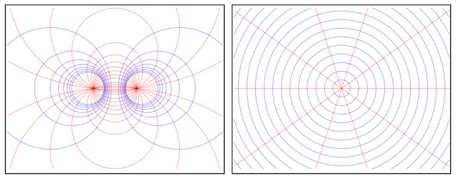
The collection of circle of Apollonius (for all possible $q$) and all circles through $a$ and $b$ form the bipolar Coordinate system induced by $a$ and $b$. Each point on the complex plane except $a$ and $b$ is the intersection of exactly one circle of Apollonius and one circle through $a$ and $b$ (see Figure 1, left).
That means that points can be uniquely identified by their corresponding Apollonius and one circle through $a$ and $b$, and so this forms a coordinate system, known as the bipolar coordinate.
Why bother with such a convoluted way to identify the position of points? In the same way that polar coordinates can be make some problems simpler, we can use the bipolar coordinates to simplify things. For this post in particular we’ll focus on its application for Möbius transformations.
Symmetry Points of a Circle
First we connect the bipolar system, in particular the circle of Apollonius, with symmetry points of a circle:
Theorem 1. Let $C$ be the circle of Apollonius corresponding to foci $a$ and $b$ and ratio $q$. Points $a$ and $b$ form a pair of symmetric points with respect to $C$.
We want to show that the identity of cross-ratios $(a, f, u, v) = \overline{(b, f, u, v)}$ holds, and then Theorem 2 in [2] would show that $a$ and $b$ are symmetric with respect to $C$.
For ease of reasoning, we can assume that $a$ and $b$ lie on the real axis (and hence also $u$ and $v$). This should not be an issue since we can apply a Möbius transformation to achieve this result and cross-ratios are invariant with Möbius transformations. We have that: $$(1.1) \quad (a, p, u, v) = \frac{a - u}{a - v} \cdot \frac{p - u}{p - v}$$ and $$\overline{(b, p, u, v)} = \frac{\overline{b - u}}{\overline{b - v}} \cdot \frac{\overline{p - u}}{\overline{p - v}}$$ Since $b, u$ and $v$ are on the real line, they're equal to their conjugates, so $$ = \frac{b - u}{b - v} \cdot \frac{\overline{p} - u}{\overline{p} - v}$$ We first show that: $$(1.2) \quad \frac{a - u}{a - v} = - \frac{b - u}{b - v}$$ Since $u$ and $v$ are points on the Apollonius circle, they satisfy $\abs{a - u} = q \abs{b - u}$ and $\abs{a - v} = q \abs{b - v}$. And since $a, b, u$ and $v$ are collinear, we have $(a - u) = -q(b - u)$ and $(a - v) = q(b - v)$. Note that since $u$ is in between $a$ and $b$, $(a - u)$ and $(b - u)$ point in opposite directions, so we need the negative $q$. So $$ \frac{a - u}{a - v} = \frac{-q(b - u)}{q(b - v)} = - \frac{b - u}{b - v} $$ Now we show that: $$(1.3) \quad \frac{p - u}{p - v} = - \overline{\left( \frac{p - u}{p - v} \right)} = - \frac{\overline{p} - u}{\overline{p} - v}$$ We consider $(p - u)$ in polar form as $R_u e^{i\theta_u}$ and $(p - v)$ as $R_v e^{i\theta_v}$. We first claim that $\theta_u - \theta_v = \pi/2$. This can be proven from the Thales Theorem which says that if $uv$ is the diameter of a circle $C$, then the angle $u \hat p v$ is $90^{\circ}$. Consider Figure 1.1:
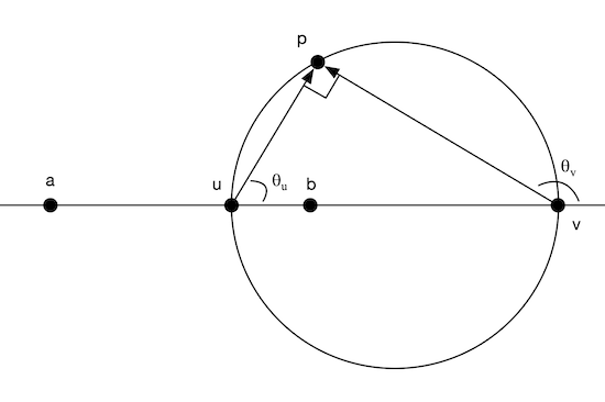
We have that $\theta_u + 90^{\circ} = (180^{\circ} - \theta_v) = 180^{\circ}$ so $\theta_u - \theta_v = 90^{\circ} = \pi/2$. So: $$\frac{p - u}{p - v} = \frac{R_u}{R_v} e^{i (\theta_u - \theta_v)} = \frac{R_u}{R_v} e^{i \pi/2}$$ If we recall that if $z = R e^{i\theta}$ then $\overline{z} = R e^{-i\theta}$, the conjugate of the above is: $$\overline{\left( \frac{p - u}{p - v} \right)} = \frac{R_u}{R_v} e^{-i \pi/2}$$ We have $-\pi/2 = 2\pi - \pi/2 = \pi + \pi/2$ and that $e^{i\pi} = -1$ (Euler's identity!), so $$\frac{R_u}{R_v} e^{-i \pi/2} = \frac{R_u}{R_v} e^{i \pi} e^{i \pi/2} = -\frac{R_u}{R_v} e^{i \pi/2}$$ Which proves $(1.3)$. Multiplying $(1.2)$ and $(1.3)$ together gives us: $$\frac{a - u}{a - v} \cdot \frac{p - u}{p - v} = \frac{b - u}{b - v} \cdot \frac{\overline{p} - u}{\overline{p} - v}$$ Showing that $(a, p, u, v) = \overline{(b, p, u, v)}$. Which proves that $a$ and $b$ are symmetric with respect to $C$.
Theorem 1 combined with Theorem 9 in [2], tell us that any circles through $a$ and $b$ must then intersect $C$ orthogonally.
Corollary 2. Circles through $a$ and $b$ intersect Apollonious circles induced by $a$ and $b$ orthogonally.
Möbius Transformation
Fixed points
In our post Möbius Transformations [3] we discussed the concept of fixed points. To recap, given a transformation $T$, a fixed point is such that $\gamma = T(\gamma)$. In the general case a Möbius transformation has two fixed points. It can have a single one, but we’ll ignore that case in this post.
Now let $a$ and $b$ be the fixed points of a Möbius transformation $T$ and consider the bipolar coordinates induced by these $a$ and $b$. What happens if we transform this system via:
\[(1) \quad z = U(w) = \frac{w - a}{w - b}\]It will send point $a$ to 0 and $b$ to $\infty$. What does it do to a Apollonius circle? Theorem 3 answers that:
Theorem 3. Transformation $U(w)$ maps Apollonius circles to circles at the origin.
How about circles through $a$ and $b$? Theorem 4 has the answer:
Theorem 4. Transformation $U(w)$ maps circles through $a$ and $b$ to lines through the origin (radial lines).
The angle of this line will be determined by any other point on the circle $C$.
Taken together, we see that transformation $U(w)$ maps a bipolar coordinate system into a polar one! A fixed Apollonius circle in the transformed plane denotes a fixed radius $r$ and a fixed circle through $a$ and $b$ in the transformed plane denotes a angle $\theta$. Figure 1 illustrates this.
Another way to prove Corollary 2 is by observing that the lines through the origin intersect circles through the origin orthogonally. Since Möbius transformations are conformal maps (Theorem 3 in [3]), the corresponding curves in the bipolar coordinates must also intersect orthogonally.
Normal Form
Recall from our post Möbius Transformations [3] that a given Möbius Transformation $T$ with fixed points $a$ and $b$ has the following normal form:
\[\frac{f(z) - a}{f(z) - b} = r e^{i\theta} \frac{z - a}{z - b}\]Taking $U(w) = (w - a)/(w - b)$, we can rewrite it as:
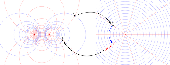
\[w' = U^{-1} ( r e^{i\theta} U(w) )\]The bipolar coordinate system gives us a more intuitive interpretation of this equation. First we map a point $w$ from the coordinate system into the polar one via $U(w)$.
In there, we multiply it by a factor of $r$ (moving it to another circle through the origin) and a rotation by $\theta$ (moving it to another radial line).
Finally we transform the resulting point back to the bipolar coordinate system by applying $U^{-1}(z)$ to the transformed point. Figure 2 illustrates this process:
Conclusion
In [1] Ahlfors calls the bipolar coordinate system a circular net or Steiner circles but I didn’t find this used on the web, except for [6].
After reading the corresponding chapter on this in [1], I didn’t fully grasp how this bipolar coordinate is useful in the context of Möbius transformations. Only after reading [5] and seeing diagrams (on which Figure 2 is based) that I got the idea and it’s really elegant, so I’m glad I took the time to complement my studies.
References
- [1] Complex Analysis - Lars V. Ahlfors
- [2] NP-Incompleteness - Symmetry Points of a Circle
- [3] NP-Incompleteness - Möbius Transformation
- [4] Geometry with an Introduction to Cosmic Topology - 3.5: Möbius Transformations: A Closer Look.
- [5] Introduction to Groups and Geometries - David W. Lyons
- [6] NP-Incompleteness - Circles of Apollonius
