kuniga.me > NP-Incompleteness > Complex Numbers and Geometry

Complex Numbers and Geometry

02 Oct 2023

In this post we’ll study some connections between complex numbers and geometry. We’ll cover the complex plane and look at complex numbers as 2-dimensional vectors with a special multiplication. We’ll provide an implementation to render the Mandelbrot fractal and finally introduce the Riemann sphere.

The Complex Plane

As we’ve seen in [1] there’s a straightforward bijection between $\mathbb{C}$ and $\mathbb{R}^2$, so the set of complex numbers can be organized as a 2-dimensional Cartesian plane, conventionaly with the x-axis representing the real part and the y-axis the imaginary part. Such plane is known as the complex plane [2]. More precisely, a complex number $z = a + ib$ corresponds to the point $(a, b)$ in the cartesian plane.

Polar Coordinates

Point in a cartesian plane can be represented in cartesian coordinates or polar coordinates. So a point with cartesian coordinates $(a, b)$ can be mapped into one with polar coordinates $(r, \theta)$ as follows:

and conversely,

For complex numbers, if we write it using the polar coordinates we get:

Which by Euler’s formula is:

Since $\abs{z} = \sqrt{a^2 + b^2} = r$, we get:

Complex Number or 2D Vector?

As it’s implied with the complex plane, a complex number of the form $z = a + ib$ can be thought as a 2D vector $(a, b) \in \mathbb{R}^2$. A lot of vector operations are valid for complex numbers:

Addition/Subtraction. is done element-wise, so given $z_1 = a_1 + i b_1$ and $z_2 = a_2 + i b_2$, we can have

And analogously for subtraction.

Length. the length of a vector $v = (a, b)$, denoted as $\abs{v}$, is defined as $\sqrt{a^2 + b^2}$, which is exactly the same definition as the modulus of a complex number:

Multiplication. multiplication is where the departure with traditional vectors starts. In linear algebra, we can have element-wise product (Hadamard product), dot product or cross product. But we can also define a new “product” as follows:

This will then match the definition of complex product:

Division division can be defined as the inverse of multiplication, so it’s not coupled with any definition of multiplication. If we want to compute $z_1 / z_2 = z_3$, we can instead do $z_1 = z_3 * z_2$ and we obtain two equations (one for each dimension):

We are interested in computing $z_3 = (a_3, b_3)$, so we can solve the equations, first for $a_3$ by isolating $b_3$:

Replacing $b_3$:

Distributing terms:

Isolating $a_3$:

Now we solve for $b_3$:

Replacing $a_3$:

Distributing terms:

Isolating $b_3$:

So

or, using $\abs{z_2}^2 = ^2_2 + b^2_2$:

In Polar Coordinates. If we use polar coordinates, we can simplify the notation by leveraging properties of $\sin$ and $\cos$. For multiplication,

If we used polar coordinates for $z_1 = (r_1 \cos \theta_1, r_1 \sin \theta_1)$ and $z_2 = (r_2 \cos \theta_2, r_2 \sin \theta_2)$:

We can use the trigonometry identities [3]:

and simplify the product to:

For division we saw that:

In polar coordinates:

using that $\sin -x = - \sin x$ we have the relations:

And can simply the division to:

So for multiplication, we multiply the magnitudes and add the angles and for division we divide the magnitudes and substract the angles. Pretty neat!

One point to emphasize is that if we work with this special definition of multiplication, we can decouple it completely from any concept of complex numbers!

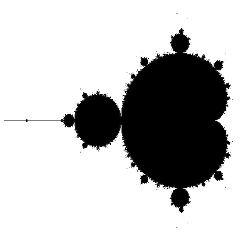
Mandelbrot Set

We can’t talk about the complex plan and leave out the Mandelbrot Set, probably the most famous fractal out there. Let $f_c(z) = z^2 + c$, where $z$ and $c$ are complex numbers.

The Mandelbrot set corresponds to all complex numbers $c$ for which recursively applying $f_c$ starting with $f_c(0)$, does not diverge, that is $\dots f_c(f_c(f_c(0))) < \infty$. If we plot these numbers in the complex plan, they form a beautiful fractal!

Since we need to render these on a computer, we need to approximate things. First is that we use a discrete number of points, corresponding to pixels on the image. Second, we can’t determine whether a complex number belongs to the Mandelbrot set analytically and we can’t perform the recursion ad infinitum, so we need cap the number of iterations to a maximum and make the call if it diverges by them.

Finally the “famous” part of the rendering is confined to a specific domain. Wikipedia [4] suggests $-2.00 \le x \le 0.47$ and $-1.12 \le y \le 1.12$. Changing these boundaries is equivalent to panning and zooming into the image.

Let’s write a code in Python for this. We’ll use numpy’s array because they have convenient element-wise operations. First we’ll define our custom multiplication function as described in the section Complex Number or 2D Vector?:

import numpy as np
def complex_mult(a, b):
  x = a[0] * a[1] - b[0] * b[1]
  y = b[0] * a[1] + a[0] * b[1]
  return np.array([x, y])

Numpy arrays don’t have a built-in function to compute a vector length (norm) but there’s one in the linear algebra sub-module, so we can define one for convenience:

def norm(a):
  return np.linalg.norm(a)

We can now define the is_in_mandelbrot_set() function:

# Maps v in [0, 1] linearly to [a, b]
def scale(v, a, b):
  return v * (b - a) + a

def scale_x(x):
  return scale(x, -2.00, 0.60)

def scale_y(y):
  return scale(y, -1.12, 1.12)

def is_in_mandelbrot_set(x, y, width, height):
  c = np.array([scale_x(x / width), scale_y(y / height)])
  def f_c(z):
    return complex_mult(z, z) + c

  z = np.zeros(2)
  n = 0
  while n < MAX_IT:
    z = f_c(z)
    if norm(z) > MAX_NORM:
      return False
    n += 1

  return True

Here MAX_IT is the maximum number of iterations we wish to perform and MAX_NORM is the threshold above which we considered a value diverged. Wikipedia [4] suggests MAX_NORM = 4 and MAX_IT = 1000.

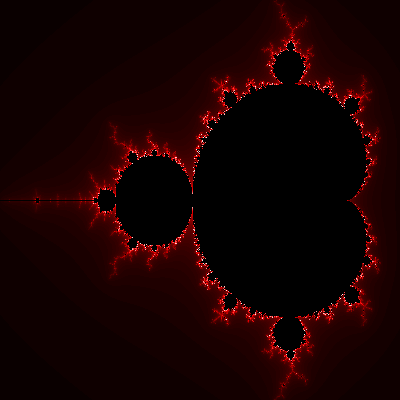
If we assign colors based on the number of iterations it took each pixel to cross the threshold MAX_NORM, we get the more usual Mandelbrot fractal. More precisely, let $N$ be the total number of iterations, and $n$ the iteration which crosses the threshold. We compute the ratio $n / N$ and use the HSL color scheme to generate a gradient in the interval $[0, 1]$.

Stereographic projections

Imagine the surface of the unit 3D sphere with its center at the origin, that is,

Now consider the intersection with the 2D plane $z = 0$. The result is the circumference of the unit circle:

We’ll assume the plane in this case is the complex plane and we’ll map each point $p$ on the surface of the sphere to a point $p’$ in the complex plane.

Borrowing some cartographic terminology, we’ll call the highest point in the sphere, i.e. $(0, 0, 0.5)$, the north pole. Now consider the line going through that north pole and $p$, which we denote by $\ell_p$. Point $p’$ will be the point where this line intersects the complex plane.

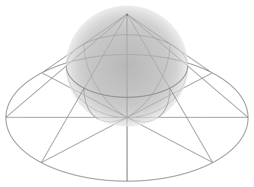
Let’s visualize 4 scenarios:

1) When $p$ has $z = 0$: then it lies on the equator of the surface of the sphere and that’s also where the line $\ell_p$ intersects the complex plane, so $p’ = p$.

2) When $p$ is below the equator: then the line $\ell_p$ intersects the complex plane inside the unit circle. In particular, if we take $p$ as the south pole, i.e. $p = (0, 0, -0.5)$, then $p’ = (0, 0)$.

3) When $p$ is above the equator: then the line $\ell_p$ intersects the complex plane outside the unit circle and the further north we move, the further out from the origin $p’$ moves.

4) Is the degenerate case where $p$ coincides with the north pole itself. There’s no unique line that passes through them so the mapping is undefined. We can treat this case specially by adding an extra element to the set of complex numbers $\mathbb{C}$, which is denoted as $\infty$ as an allusion to the fact that the norm of $p’$ tends to infinity as $p$ tends to the north pole.

The set $\mathbb{C} \cup \infty$ is called the extended complex numbers and the surface of the sphere is known as the Riemann sphere [5] (I’m not sure why it’s called just sphere given it only includes the surface).

The actual mapping can be given as follows. Let $(x_1, x_2, x_3)$ be a point on the surface of the sphere and $z$ a complex number. Then,

To obtain the reverse mapping, we first observe that:

Since the point is on the surface of the unit sphere, we have $x_1^2 + x_2^2 + x_3^2 = 1$, so $x_1^2 + x_2^2 = 1 - x_3^2 = (1 + x_3)(1 - x_3)$,

Isolating $x_3$ gives us

Since $x_1, x_2, x_3 \in \mathbb{R}$, $\Re(z) = \frac{x_1}{1 - x_3}$. Using the identity $\Re(z) = \frac{z + \bar{z}}{2}$,

By (2), we have that $1 - x_3 = \frac{2}{\abs{z}^2 + 1}$, so

Similarly for $x_2$, we have that $\Im(z) = \frac{x_2}{1 - x_3}$. Using the identity $\Im(z) = \frac{z - \bar{z}}{2i}$,

Note that (1) is not defined for the north pole $(0, 0, 1)$, in which case we explicitly map is to $z = \infty$.

Conclusion

This post is a complement to my studies of the book Complex Analysis by Lars V. Ahlfors. I was already relatively familiar with the complex plane and polar coordinates, but I don’t recall ever looking into the implementation of the Mandelbrot fractal. It does feel like something I’d have to implement in college, so maybe I’m just forgetting?

I had only heard of the Riemann sphere in passing but never stopped to learn about it. It’s actually not that complicated but I don’t quite grasp yet why it’s useful.

Related Posts

The Cardinality of Complex Numbers. In that post we showed there is a 1:1 mapping between $\mathbb{R}$ and $\mathbb{R}^2$. This result also gives us a 1:1 mapping between $\mathbb{R}^3$ and $\mathbb{R}^2$ and hence $\mathbb{C}$. Now, the surface of the unit sphere is definitely contained in $\mathbb{R}^3$ but the stereographic projection says there’s one point (the north pole) in that surface that doesn’t have a correspondent in $\mathbb{C}$! This is an example of how counter-intuitive mappings involving set of infinite sizes are.

Random Points in Circumference. Let’s recap that post: to generate random points in a circumference, we first generate a pair of floating numbers $(X, Y)$ such that $0 \lt X^2 + Y^2 \le 1$. This can be done by generating $X$ and $Y$ uniformily and independently and discarding pairs not satisfying that constraint.

This pair lies inside the unit circle, but we want to have them in the circumference. We can do this by dividing the number by its norm:

But this involves computing the square root. Von Neumann devised a way to avoid it by showing that:

also generates a random point in a circumference. If we set $Z = (X, Y)$, the numerators of these fractions are exactly $Z * Z$! Given $\abs{Z} = \sqrt{X^2 + Y^2}$, we can express it much more succinctly in complex numbers:

Let’s understand why this works. We know that $Z / \abs{Z}$ is a point on the circumference of unit circle in the complex plane. We also know that multiplying two complex numbers corresponds to adding their angles in polar coordinates, and more specifically squaring a complex number is doubling its angles.

The argument we used in that post is that because the angle is continuous and periodic, generating a point with twice the angle does not break the uniformity of the distribution.

Z-Transform. Complex numbers are very useful in signal processing, so not surprisingly we see the use of the complex plane. For Z-transform in particular, we use the complex plane and the unit circle to display poles and zeros of the transfer function.

Discrete Fourier Transforms. In this post we provide some intuition on why complex numbers are used in real-world applications:

What does a complex number refer to in the real world? The insight provided by [1] is that $\mathbb{C}$ is just a convenient way to represent 2 real-valued entities. We could work with $\mathbb{R}^2$ all along, but the relationship between the two entities is such that complex numbers and all the machinery around it works neatly for signals.

This is inline with the observation we made above in Complex Number or 2D Vector?:

One point to emphasize is that if we work with this special definition of multiplication, we can decouple it completely from any concept of complex numbers!

References

• [1] NP-Incompleteness - The Cardinality of Complex Numbers
• [2] Wikipedia - Complex plane
• [3] NP-Incompleteness - Trigonometry Cheat Sheet
• [4] Wikipedia - Plotting algorithms for the Mandelbrot set
• [5] Wikipedia - Riemann sphere

Source code | RSS feed | Tags: analysis