kuniga.me > NP-Incompleteness > Random Points in Circumference
Random Points in Circumference
01 Aug 2022
I recently wanted to generate points in the circumference of a unit circle. After some digging, I found a very elegant algorithm from John von Neumann and then a related method for generating normally distributed samples.
In this post we’ll describe these methods starting with a somewhat related problem which provides some techniques utilized by the other methods.
$\pi$ From Random Number Generator
First, let’s explore a different problem: how can we estimate $\pi$ using only a random number generator? The idea is to define a point with independent random variables as coordinates $(X, Y)$, uniformed sampled from $[-1, 1]$.
Suppose we sampled values $x$ and $y$. Then we compute the fraction of samples such that $x^2 + y^2 \le 1$. We claim that this ratio will be approximately $\frac{\pi}{4}$!
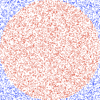
The idea is that when $x^2 + y^2 \le 1$ they’re points inside the unit circle (centered in 0). Whereas $(x, y)$ are coordinates of a square of side 2. Since the samples are uniformly distributed, we’d expect that the proportion of points inside the circle over the total will be the ratio of the area of the circle, $\pi r^2$ over that of the square, $\ell^2$. Since $r = 1$ and $\ell = 2$, we get $\frac{\pi}{4}$, which is approximately 0.78.
To gain better intuition, we can plot the points. We color the ones satisfying $x^2 + y^2 \le 1$ red, otherwise blue. Figure 1 shows an example with 10,000 samples.
I learned about this trick many years ago from Brain Dump (in Portuguese).
Random Points in Circumference
Now let’s focus on our main problem. One naive idea to solve it using the method we just saw above is to generate sample points and discard all those not satisfying $x^2 + y^2 = 1$. This would be incredibly inefficient and in theory the probability of a continuous random variable is actually 0.
Another approach is to generate a random number $\Theta$ in the interval $[0, 2 \pi[$. We can then compute $x = \cos \Theta$ and $y = \sin \Theta$ which will be in the circumference. It’s possible however to avoid computing $\sin$ and $\cos$ altogether, with a method proposed by von Neumann [1].
First we generate a random point inside the unit circle. We just saw how to do this above: define random variables $X$ and $Y$, uniformly sampled from $[-1, 1]$. Discard sample if $X^2 + Y^2 > 1$.
Recall that we can represent a point in cartesian coordinates $(X, Y)$ with polar coordinates $(R, \Theta)$, where $X = R \cos \Theta$ and $Y = R \sin \Theta$ and $R = \sqrt{X^2 + Y^2}$.
If $X$ and $Y$ are random points in the unit circle, $\Theta$ is uniformly distributed over the interval $[0, 2 \pi[$. Intuitively, there’s no reason to assume a given angle is more likely if we pick a point at random inside a circle. Notice this is not true if we sample inside a square!
If we wish to generate coordinates $(X’, Y’)$ on the circumference of the unit circle, we can compute $X’ = \cos \Theta$, which can be obtained as
\[X' = \cos \Theta = \frac{X}{R} = \frac{X}{\sqrt{X^2 + Y^2}}\]Similarly for $Y’ = \sin \Theta$:
\[Y' = \sin \Theta = \frac{Y}{R} = \frac{Y}{\sqrt{X^2 + Y^2}}\]Computing the square root is not ideal, so the trick is to use $2\Theta$ which is uniformly sampled between $[0, 4 \pi[$, but since trigonometric functions have period $2\pi$ (e.g. $\sin(x) = \sin(x + 2 \pi)$ and $\cos(x) = \cos(x + 2 \pi)$), effectively $2\Theta$ has the same distribution as $\Theta$!
Assuming $X’ = \cos(2\Theta)$ and using the identity $\cos(2\Theta) = \cos \Theta^2 - \sin \Theta^2$:
\[X' = \frac{X^2 - Y^2}{R^2} = \frac{X^2 - Y^2}{X^2 + Y^2}\]Similarly $Y’ = \sin(2\Theta) = 2 \sin(x) \cos(x)$:
\[Y' = \frac{2XY}{R^2} = \frac{2XY}{X^2 + Y^2}\]Which gets rid of the square root! We have to be careful with small values of $X^2 + Y^2$ in the denominator, but we can discard points when $X^2 + Y^2 \le \epsilon$ without affecting the distribution of $\Theta$.
Experimentation
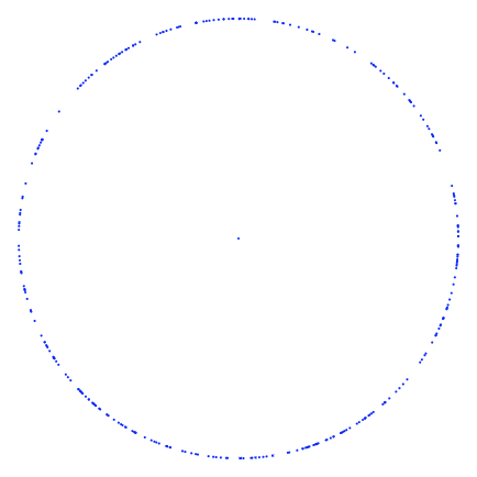
We can generate multiple points using this method and plot them in the plane to obtain Figure 2.
Complexity
The probability of a point falling inside the circle is $\frac{\pi}{4}$, so the number of tries until we find a valid point can be modeled as a geometric distribution with success rate $p = \frac{\pi}{4}$, with expected value given by $\frac{1}{p} = \frac{4}{\pi} = 1.27$, which is pretty efficient.
Amazingly, it’s possible to use this technique to generate points with a normal distribution, as we’ll see next!
Generating Normal Distribution
If a random variable $X$ has a normal distribution ($\sigma = 1$, $\mu = 0$), its cumulative probability distribution (CDF) can be given by:
\[(1) \quad P(X \le x) = F_X(x) = \sqrt{\frac{1}{2\pi}} \int_{-\infty}^{x} e^{-u^2/2} du\]Now, consider a random point $(X, Y)$ inside the unit circle. We define
\[(2) \quad N_1 = X \sqrt{\frac{-2 \ln S}{S}}\] \[(3) \quad N_2 = Y \sqrt{\frac{-2 \ln S}{S}}\]Where $S = X^2 + Y^2$. We’ll show that $N_1$ and $N_2$ are normally distributed independent variables.
As before, we represent $(X, Y)$ in polar coordinates $(R, \Theta)$, where $X = R \cos \Theta$ and $Y = R \sin \Theta$, $R = \sqrt{X^2 + Y^2}$ and thus $S = R^2$.
We can write (2) as
\[N_1 = \frac{X}{R} \sqrt{-2 \ln S} = \cos \Theta \sqrt{-2 \ln S}\]and (3) as:
\[N_2 = \frac{Y}{R} \sqrt{-2 \ln S} = \sin \Theta \sqrt{-2 \ln S}\]The pair $(N_1, N_2)$ forms a cartesian coordinate so they too can be written in polar form: $N_1 = R’ \cos\Theta’$ and $N_2 = R’ \sin\Theta’$, for $R’ > 0$ and $\Theta’ \in [0, 2 \pi[$.
Every cartesian coordinate can be uniquely represented in a polar form as $\alpha \sin(\phi)$ and $\alpha \cos(\phi)$, if $\alpha > 0$ and $\phi \in [0, 2 \pi[$. So if we ignore samples with $S = 0$ (making $\sqrt{-2 \ln S} > 0$) and we can normalize $\Theta$ to be $\in [0, 2 \pi[$, this allows us to conclude that $R’ = \sqrt{-2 \ln S}$ and $\Theta’ = \Theta$.
Let’s compute the CDF for $R’$, i.e. the probability that $R’ \le r$. Since $R’ = \sqrt{-2 \ln S}$, we need to find $-2 \ln S \le r^2$ or $\ln S \ge -r^2/2$. Applying $\exp()$ on both sides yields: $S \ge e^{-r^2/2}$.
We claim that $S$ is uniformly distributed in the range $0 \le x \le 1$ (see Appendix for proof). Thus $P(S \le e^{-r^2/2}) = e^{-r^2/2}$ and since $P(S \ge e^{-r^2/2}) = 1 - P(S \le e^{-r^2/2})$ we have $P(R’ \le r) = 1 - e^{-r^2/2}$.
The probability $R’$ is in the interval $[r, r + dr]$ can be obtained by the derivative $d\frac{P(R’ \le r)}{dr}$, which is $re^{-r^2/2} dr$.
$\Theta’$ is uniformly distributed in the range $[0, 2 \pi[$, so its CDF is $F_{\Theta’}(\theta) = \frac{\theta}{2 \pi}$ and the probability $\Theta’$ is in the interval $[\theta, \theta + d\theta]$ is $d\frac{F_{\Theta’}(\theta)}{d\theta} = (1/2\pi)d\theta$.
Because $R’$ and $\Theta’$ are independent variables, we can compute their joint probability more easily, since:
\[P(R' = r, \Theta' = \theta) = P(R' = r) P(\Theta' = \theta) = re^{-r^2/2} dr (1/2\pi)d\theta\]Thus, to compute the CDF over an interval:
\[P(R' \le r', \Theta' \le \theta') = \int_{0}^{r'} re^{-r^2/2} dr \int_{0}^{\theta'} (1/2\pi) d\theta = \frac{1}{2\pi} \int_{0}^{r'} \int_{0}^{\theta'} re^{-r^2/2} dr d\theta\]A further generalization is to combine both integrals into one but sum over a pair $(r, \theta)$ based on a predicate:
\[\frac{1}{2\pi} \int_{0}^{r'} \int_{0}^{\theta'} re^{-r^2/2} dr d\theta = \frac{1}{2\pi} \int_{(r, \theta): r \le r', \theta \le \theta'} re^{-r^2/2} dr d\theta\]This predicate-based integral over a pair form is convenient for what we’ll do next. We now want to compute the joint probability $P(N_1 \le x_1, N_2 \le x_2)$ which can be expressed in polar form:
\[P(N_1 \le x_1, N_2 \le x_2) = P(R' \cos\Theta' \le x_1, R' \cos\Theta' \le x_2)\]The predicate-based integral over $(r, \theta)$ is useful for this because while $R’$ and $\Theta’$ are independent, the conditions $R’ \cos\Theta’ \le x_1$ and $R’ \cos\Theta’ \le x_2$ are binding them together, thus we can do:
\[P(R' \cos\Theta' \le x_1, R' \cos\Theta' \le x_2) = \frac{1}{2\pi} \int_{(r, \theta): r \cos \Theta \le x_1, r \sin \Theta \le x_2} re^{-r^2/2} dr d\theta\]We can switch from polar coordinates to cartesian:
\[= \frac{1}{2\pi} \int_{(x, y): x \le x_1, y \le x_2} re^{-(x^2 + y^2)/2} dx dy\]In this form we can switch back to the interval-based integrals:
\[= \frac{1}{2\pi} \int_{-\infty}^{x_1} \int_{-\infty}^{x_2} re^{-(x^2 + y^2)/2} dx dy\]Which can be split into a product of integrals:
\[= \frac{1}{2\pi} \left(\int_{-\infty}^{x_1} re^{-x^2/2}dx\right) \left(\int_{-\infty}^{x_2} re^{-y^2/2}dy\right)\]Moving the $1 / 2\pi$ in equal parts to each factor yields:
\[P(N_1 \le x_1, N_2 \le x_2) = \left(\sqrt{\frac{1}{2\pi}} \int_{-\infty}^{x_1} re^{-x^2/2}dx\right) \left(\sqrt{\frac{1}{2\pi}} \int_{-\infty}^{x_2} re^{-y^2/2}dy\right)\]Each factor now represents the CDF for a normal distribution as in (1)! And since the factors are separable their distributions are independent:
\[P(N_1 \le x_1, N_2 \le x_2) = P(N_1 \le x_1) P(N_2 \le x_2)\]So if we want to generate a normally distributed random value we can generate a sample $(x, y)$ in the unit circle and compute a number with either (2) or (3).
This method was devided by Box, Marsaglia and Muller [2] and is known as the Polar Method.
Experimentation
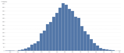
We can generate multiple points using (2) or (3) and build a histogram as in Figure 3. Note the bell-shaped curve which is what we’d expect from sampling from a normal distribution.
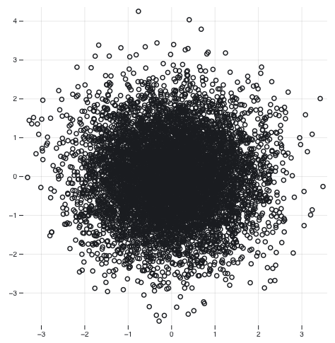
We can also generate points $(x, y)$ with $x$ sampled from (2) and $y$ from (3) and plot them in a scatterplot to visualize their correlation as in Figure 4. Notice that the circle shape suggests the distributions used to generate the samples are not correlated.
Conclusion
The process of investigating the question of generating points on the circumference let me to very interesting findings. I first found an article at MathWorld which provides the formula for the generator but not the theory behind it. It refers to a paper from von Neumman which luckily was available online but somewhat hard to understand.
In another search attempt I ran into a Q&A (I forgot the link) where the OP mentioned Knuth’s TAOCP and looking it up led me to find the normally distribution sample via the polar method, which in turn made it easier to understand von Neumann’s method.
Appendix
Lemma 1. $S$ is uniformly distributed in the range $0 \le r \le 1$.
First we compute the CDF $P(R \le r)$ for $r \in [0, 1]$. The odds we pick a point which falls with a circle of radius $r$ is the ratio of the area of such circle over the area of the unit circle, that is,
\[(4) \quad P(R \le r) = \frac{\pi r^2}{\pi} = r^2\]We now compute $P(S \le r)$ for $r \in [0, 1]$. Since $S = R^2$ we have $P(S \le r) = P(R^2 \le r) = P(-\sqrt{r} \le R \le \sqrt{r})$.
Since $R$ represents the radius, $R \ge 0$ and thus $P(R \le 0) = 0$, so $P(R \le -\sqrt{r}) = 0$ and $P(-\sqrt{r} \le R \le \sqrt{r}) = P(R \le \sqrt{r})$. From (4) we get
\[P(S \le r) = P(R \le \sqrt{r}) = r\]Which is the CDF for uniform distribution. QED.
References
- [1] Various Techniques Used in Connection With Random Digits, J. von Neumann.
- [2] The Art of Computer Programming: Volume 2, 3.4.1, D. Knuth. (p. 122)
