kuniga.me > NP-Incompleteness > Z-Transform
Z-Transform
10 Sep 2021
In this post we’ll learn about the Z-transform. This is the continuation of the study of Discrete Filters, so it’s highly recommended to check that post first.
Constant-Coefficient Difference Equations
A more general form of a discrete filter is
\[\sum_{k = -\infty}^{\infty} a_k y_{t-k} = \sum_{k = -\infty}^{\infty} b_k x_{t-k}\]In Discrete Filters, we had $a_0 = 1$ and the rest of $a$’s equal to $0$, leading to:
\[y_{t} = \sum_{k = -\infty}^{\infty} b_k x_{t-k}\]And if we say $\vec{b}$ is the impulse response $\vec{h}$, we get the definition of convolution $\vec{y} = \vec{x} * \vec{h}$.
Now suppose only $a_0 = 1$, but we assume nothing of the rest, so we have:
\[(1) \qquad y_{t} = \sum_{k = -\infty}^{\infty} b_k x_{t-k} - \sum_{k = -\infty, k \ne 0}^{\infty} a_k y_{t-k}\]Which we can interpret as the current output depending on previous ones. This is known as a Constant-Coefficient Difference Equation or CCDE.
Z-Transform
The Z-transform is a function of a vector $\vec{x}$ and a complex variable $z \in \mathbb{C}$ and defined as:
\[(2) \qquad \mathscr{Z}(\vec{x}, z) = \sum_{t = -\infty}^{\infty} x_t z^{-t}\]If we set $z = e^{i \omega}$ for $0 \le \omega \le 2 \pi$ we get the Discrete-Time Fourier Transform, so we can think of the Z-transform as an abstraction.
According to [1], Z-transform doesn’t have a physical interpretation like the DTFT does, but it’s useful as a mathematical tool.
Properties
Linearity. Given vectors $\vec{x}, \vec{y}$ and scalars $\alpha, \beta$, the Z-transform satisfies:
\[\mathscr{Z}(\alpha \vec{x} + \beta \vec{y}, z) = \alpha \mathscr{Z}(\vec{x}, z) + \beta \mathscr{Z}(\vec{y}, z)\]Time-shift. Let $\vec{x}$ be a vector and $\vec{x}’$ another vector corresponding to the entries in $\vec{x}$ shifted by $N$ positions, that is, $x’_t = x_{t-N}$. Then the Z-transform satisfies:
\[\mathscr{Z}(\vec{x}', z) = z^{-N} \mathscr{Z}(\vec{x}, z)\]It follows that
\[(3) \qquad z^{-N} \mathscr{Z}(\vec{x}, z) = \sum_{t = -\infty}^{\infty} x_{t - N} z^{-t}\]Z-Transform on CCDEs
What happens if we apply the Z-transform to (1)? Let’s define $Y(z) = \mathscr{Z}(\vec{y}, z)$ and $X(z) = \mathscr{Z}(\vec{x}, z)$ to simplify the notation.
We have
\[Y(z) = \sum_{t = -\infty}^{\infty} y_t z^{-t}\]Replacing $y_t$ from (1):
\[Y(z) = \sum_{t = -\infty}^{\infty} \left(\sum_{k = -\infty}^{\infty} b_k x_{t-k} - \sum_{k = -\infty, k \ne 0}^{\infty} a_k y_{t-k}\right) z^{-t}\]We can re-arrange the sums to obtain:
\[Y(z) = \left(\sum_{k = -\infty}^{\infty} b_k \sum_{t = -\infty}^{\infty} x_{t-k} z^{-t} \right) - \left(\sum_{k = -\infty, k \ne 0}^{\infty} a_k \sum_{t = -\infty}^{\infty} y_{t-k} z^{-t} \right)\]We note from (3) that the inner sums are $X(z) z^{-k}$ and $Y(z) z^{-k}$ respectively:
\[Y(z) = \sum_{k = -\infty}^{\infty} b_k X(z) z^{-k} - \sum_{k = -\infty, k \ne 0}^{\infty} a_k Y(z) z^{-k}\]We can re-arrange to isolate $Y(z)$ and get:
\[Y(z) = \frac{\sum_{k = -\infty}^{\infty} b_k X(z) z^{-k}}{1 + \sum_{k = -\infty, k \ne 0}^{\infty} a_k z^{-k}}\]Since $X(z)$ is independent of $k$:
\[Y(z) = \frac{\sum_{k = -\infty}^{\infty} b_k z^{-k}}{1 + \sum_{k = -\infty, k \ne 0}^{\infty} a_k z^{-k}} X(z)\]We define the first multiplier as $H(z)$, known as the transfer function of the filter described by the CCDE:
\[Y(z) = H(z) X(z)\]The transfer function is the Z-transform of the impulse response of the filter. To see why, recall that to obtain the impulse response of a system we set $\vec{x} = \vec{\delta}$ when computing $\vec{y}$. It’s easy to see that $X(z) = \mathscr{Z}(\vec{\delta}, z) = 1$, so $Y(z) = H(z)$.
It’s thus no coincidence the choice of $H$ to denote the transfer function, since it is closely related to the impulse response $h$.
Convergence
Region of Convergence
Recall that $z$ is a complex variable, so we can “visualize” its domain as the 2D plane (complex plane). The set of values of $z$ such that the sum in (2) converges absolutely is defined as the region of convergence, or $ROC\curly{\mathscr{Z}(\vec{x}, z) }$.
We can split (2) into 2, so that both start from index 0 and define a series in the form we usually define convergence over:
\[\mathscr{Z}(\vec{x}, z) = \sum_{t = -\infty}^{-1} x_t z^{-t} + \sum_{t = 0}^{\infty} x_t z^{-t} = \sum_{t = 1}^{\infty} x_t z^{t} + \sum_{t = 0}^{\infty} x_t \frac{1}{z}^{t}\]For $\mathscr{Z}(\vec{x}, z)$ to exist, both the sums must converge. Each of them define a complex power series, that is a series of the form $\sum_{k = 0}^{\infty} c_k z^k$.
It’s possible to show (see Appendix) that given a complex power series there is $0 \le R \le \infty$ such that it converges absolutely for $\abs{z} \le R$ (absolutely if $\abs{z} < R$) and diverges for $\abs{z} > R$.
We can thus find $R$ for each of the complex power series, say $R_1, R_2$ and define the region of convergence for $\abs{z} < \min(R_1, R_2)$.
Note that region of convergence of $\abs{z}$ defines a circle when visualized in the complex plane.
Convergence and Stability
In Discrete Filters [link], we showed that for a system is bounded-input bounded-output (BIBO) if, and only if, its impulse response $\vec{h}$ to be absolutely summable.
Recall that the transfer function is the Z-transform of the impulse response of the filter:
\[H(z) = \mathscr{Z}(\vec{h}, z) = \sum_{t = -\infty}^{\infty} h_t z^{-t}\]If $H(z)$ is absolute convergent for $\abs{z} = 1$, then $\sum_{t = -\infty}^{\infty} \abs{h_t z^{-t}}$ converges, and since $\abs{a b} = \abs{a} \abs{b}$ [3], then $\sum_{t = -\infty}^{\infty} \abs{h_t} \abs{z^{-t}} = \sum_{t = -\infty}^{\infty} \abs{h_t}$ also converges.
We conclude that a system is BIBO if its ROC contains $\abs{z} = 1$.
Poles and Zeros
Realizable Filters
A filter is realizable if we can implement it via some finite algorithm, which means that $y_t$ in (1) can only depend on a finite number of terms and is causal (i.e. only depends on past terms):
\[y_{t} = \sum_{k = 0}^{M-1} b_k x_{t-k} - \sum_{k = 1}^{N-1} a_k y_{t-k}\]The transfer function for realizable filters is the ratio of finite-degree polynomials, in which case it’s also called rational transfer function:
\[H(z) = \frac{\sum_{k = 0}^{M-1} b_k z^{-k}}{1 + \sum_{k = 1}^{N-1} a_k z^{-k}}\]Poles of the Transfer Function
Since the Z-transform for realizable filters is finite, they’re convergent. However, for the transfer function to exist, we must have the denominator of $H(z)$ to be non-zero.
We thus need to find the values of $z$ for which this polynomial is zero:
\[1 + a_1 z^{-1} + a_2 z^{-2} + \cdots + a_{N-1} z^{-(N-1)}\]In other words, we want to find the roots of this polynomial, say $p_0, \cdots, p_{N-1}$, which in this context is known as the poles of the transfer function. The ROC cannot contain any poles.
Let $p^*$ be the pole with hightest magnitude. Thus if $\abs{z} > \abs{p^{*}}$ we’re guaranteed to avoid zeros in the denominator.
Moreover, if $\abs{p^*} \le 1$, there’s a region defined by $\abs{p^*} < \abs{z} \le 1$ where the system is convergent and BIBO.
Zeros of the Transfer Function
We can similarly find the root of the polynomial in the numerator of $H(z)$, say $z_0, \cdots, z_{M-1}$. We can then express the transfer function as a product of terms.
For each root $r$, we can add a factor $(z - r)$ or to keep it in terms of $z^{-1}$, $(1 - r z^{-1})$, noting both evaluate to 0 when $z = r$.
\[(4) \qquad H(z) = b_0 \frac{\prod_{k = 0}^{M-1} (1 - z_n z^{-1})}{\prod_{k = 0}^{N-1} (1 - p_n z^{-1})}\]We assume the denominator and numerator are co-prime so they can’t be called out.
The Pole-Zero Plot
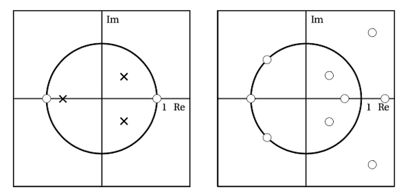
We can visualize the zeros and poles in the complex plane for $z$. The convention is to display poles as crosses (X) and zeros as dots (O).
We also overlay the unit circle because inside the unit circle the system is BIBO. We can use this plot to quickly detect if any poles lie outside of the unit circle. Figure 1 has two example filters.
If we’re to plot $\abs{H(z)}$ (z-axis) over $z$ (xy-plane) we’d have a 3D plot where for zeros, $\abs{H(z)} = 0$ and for poles $\abs{H(z)} = \infty$, visually the poles would look like, guess what… poles, hence the name.
Filtering Poles Out
When we apply a filter after another, we can get the resulting impulse response via convolution as we briefly mention in Discrete Filters.
If the impulse responses are absolute summable, we can apply the convolution theorem also described previously [4] (we proved it for DTFT but can be easily generalized for the Z-transform).
Using the convolution theorem, we have that if the impulse response of 2 filters is the convolution $\vec{h_1} * \vec{h_2}$, the combined transfer function is the product of their Z-transform $\mathscr{Z}(\vec{h_1}, z) \mathscr{Z}(\vec{h_2}, z)$.
Looking at the definition of (4), we can combine filters to remove poles from another. For example, suppose $\mathscr{Z}(\vec{h_1}, z)$ has a pole $\abs{p_i} > 1$ we want to remove. We can configure the second filter so that the numerator in $\mathscr{Z}(\vec{h_2}, z)$ contains a factor $(1 - z_j z^{-1})$ (with $z_j = p_i$) that can cancel out the factor $(1 - p_i z^{-1})$ in the denominator of $\mathscr{Z}(\vec{h_1}, z)$!
Examples
Moving Average
Recall from [4] that the moving average filter is:
\[y_t = \mathscr{H}(\vec{x}, t) = \frac{1}{N} \sum_{k = 0}^{N - 1} x_{t - k}\]So we have:
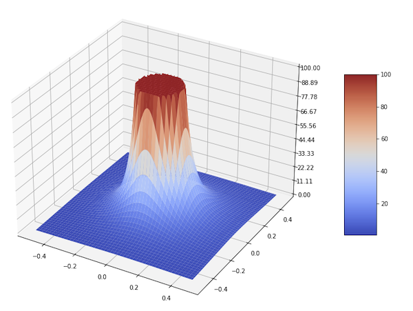
\[H(z) = \frac{1}{N} \sum_{t = 0}^{N-1} z^{-t}\]Which is a geometric series with closed form:
\[H(z) = \frac{1}{N} \frac{1 - z^{-N}}{1 - z^{-1}}\]In Figure 2 we plot $\abs{H(z)}$ (z-axis) over $z$ (xy-plane). When $\abs{z} \rightarrow 0$, then $\abs{z^{-N}} \rightarrow \infty$ so we have to crop the chart for low values of $\abs{z}$.
Let’s define $z’ = 1/z$. The roots of the numerator are the $z’$ which raised to $N$ yield 1. They’re known as root of unit and are of the form: $z’ = e^{(2 k \pi i)/N}$ for $k = 0, \cdots, N-1$.
In other words, when $z = e^{(-2 k \pi i)/N}$ for $k = 0, \cdots, N-1$, then $H(z) = 0$. Further, when $k = 0$, $z = 1$ and it cancels out the denominator. We can then write $H(z)$ as a product of roots:
\[H(z) = \frac{1}{N} \prod_{k = 1}^{N} (1 - e^{(-2 k \pi i)/N} z^{-1})\]This means the moving average filter does not have poles, but this is curious because for $z = 0$ the $\abs{H(z)}$ tends to infinity, so in that sense it does look like a pole, but it’s not a pole according to the definition.
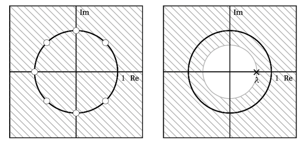
If we plot the zeros on the complex plane, we’ll have $N$ dots evenly spread out on the unit circle.
Leaky Integrator
Recall from [4] that the leaky integrator filter is:
\[y_t = \lambda y_{t - 1} + (1 - \lambda) x_t\]With $b_0 = (1 - \lambda)$ and $a_1 = -\lambda$ and all the other coefficients 0, so we have:
\[H(z) = \frac{1 - \lambda}{1 - \lambda z^{-1}}\]The pole is when $z = \lambda$, so we achieve convergence when $\abs{z} > \lambda$. Finally the the system is stable if $\lambda < 1$.
Conclusion
The main reason I picked up the book from Prandoni and Vetterli [1] was to learn about the Z-transform. I was trying to learn about some other DSP topic and a lot of the ideas were over my head, and I realized I needed a better foundation. The region of convergence of the transfer function was one of the things I couldn’t get, but I now have a much better grasp of it.
While studying this topic, I had some very vague recollections of having seen something similar to region of convergence in the unit circle during my undergraduate years. I looked up the curriculum and found EE400, which does mention complex numbers and power series, but not the Z-transform.
It’s likely it was the Laplace transform I learned about, which is the continuous version of the Z-transform [5]. Analogously, CCDEs are the discrete counterpart to differential equations. Despite the name, I didn’t make the connection, and I’d like to learn more about their similarities at some point.
The book [1] mentions in passing that when a complex power series converges it converges absolutely. Maybe it’s a well known result but it was pretty tricky for me to see why that’s the case and I had to go over several steps in the Appendix to convince myself.
This was the first time I used matplotlib’s 3D plot and it’s possibly the first time I plot a 3D chart.
Related Posts
Linear Predictive Coding in Python - While looking into translating the Matlab code into Python, I had to look up the definition of lfilter, which I couldn’t understand at the time.
The docs describe a filter in terms of the coefficients $a$ and $b$ in the CCDE form (which they call direct II transposed structure). It also mentions the rational transfer function! Everything makes much more sense now.
So when we have:
b = np.concatenate([np.array([-1]), a])
x_hat = lfilter([1], b.T, src.T).T
We’re basically describing a filter:
\[y_t = -x_{t} + \sum_{i = 1}^{n} a_i x_{t - i}\]Where $\vec{x}$ is src and $\vec{y}$ is x_hat.
Appendix
It’s worth recalling that a complex series
\[\sum_{k = 0}^{\infty} c_k, \quad \mbox{where } c_k = a_k + i b_k \in \mathbb{C}\]converges if both its real and imaginary series:
\[\sum_{k = 0}^{\infty} a_k \qquad \mbox{and} \qquad \sum_{k = 0}^{\infty} b_k\]converge. A complex series converges absolutely if the following real series converges:
\[\sum_{k = 0}^{\infty} \abs{c_k}, \qquad \abs{c_k} = \sqrt{a_n^2 + b_n^2}\]Let’s consider some lemmas.
Lemma 1. If a real series $\sum_{n = 0}^{\infty} a_n$ converges, then $\lim_{n \rightarrow \infty} \abs{a_k} = 0$.
Proof. Consider the partial sum $S_n = \sum_{k = 0}^{n} a_k$. By definition, $\sum_{k = 0}^{\infty} a_k$ is convergent if $\lim_{n \rightarrow \infty} S_n = L$ for some real $L$ and so $\lim_{n \rightarrow \infty} S_{n+1} = L$. We have that $a_{n + 1} = S_{n+1} - S_{n}$, so $\lim_{n \rightarrow \infty} a_{n + 1} = L - L = 0$. QED
Lemma 2. If a complex series converges, then $\lim_{n \rightarrow \infty} \abs{c_n} = 0$.
Proof. By definition $\sum_{n = 0}^{\infty} a_n$ and $\sum_{n = 0}^{\infty} b_n$ converge, so by Lemma 1, $\lim_{n \rightarrow \infty} \abs{a_n} = 0$ and $\lim_{n \rightarrow \infty} \abs{b_n} = 0$, thus $\lim_{n \rightarrow \infty} c_n = \sqrt{\abs{a_n}^2 + \abs{b_n}^2} = 0$. QED
Consider the following complex power series:
Lemma 3. Consider the complex power series $\sum_{n = 0}^{\infty} z^n$. If $\abs{z} < 1$ then it converges absolutely, and if $\abs{z} \ge 1$, it diverges.
Proof. If $\abs{z} < 1$, then $\sum_{n = 0}^{\infty} \abs{z}^n$ is a geometric series, which has a closed form given by
\[\frac{1 - \abs{z}^{n + 1}}{1 - \abs{z}}\]Because $\lim_{n \rightarrow \infty} \abs{z}^{n + 1} = 0$, the geometric series converges to $1 / (1 - \abs{z})$. Since $\abs{z}^n = \abs{z^n}$, it follows that $\sum_{n = 0}^{\infty} \abs{z^n}$ is convergent.
Conversely, if $\abs{z} \ge 1$, then $\abs{z^n} \ge 1 \ne 0$, so $\sum_{n = 0}^{\infty} \abs{z^n}$ must diverge otherwise it would contradict Lemma 2. QED
Lemma 4. If $\sum_{n = 0}^{\infty} a_n$ converges, then $\abs{a_n} \le M$ for all $n$.
Proof. By definition, given an arbitrary $\epsilon > 0$, there exists $L$ and $N$ such that $\abs{S_n - L} < \epsilon$ for $n \ge N$. Then $\abs{S_{n+1} - L} < \epsilon$, and we claim that $\abs{a_{n+1}} < 2 \epsilon$ because otherwise adding $a_{n+1}$ to $S_n$ would violate the constraint for $S_{n+1}$.
Now, since $N$ is finite, the upper bound $M = \max(\abs{a_n})$ for $n \le N$ is defined. It’s easy to see that $\abs{a_n} \le \max(M, 2\epsilon)$ for all $n$. QED
Consider the following complex power series:
\[(5) \quad \sum_{k = 0}^{\infty} c_k z^k, \qquad c_k, z \in \mathbb{C}\]Lemma 5. Suppose (5) converges for $z = w_0 \ne 0$. Show that if $\abs{w} < \abs{w_0}$, then (5) converges absolutely for $z = w$.
Proof. We can write $\abs{c_n w^n}$ as:
\[\abs{c_n w^n} = \abs{c_n w_0^n \frac{w^n}{w_0^n}} = \abs{c_n w_0^n} \abs{\frac{w^n}{w_0^n}} = \abs{c_n w_0^n} \abs{\frac{w}{w_0}}^n\]Since (5) is convergent, by Lemma 4, there exists $M$ such that $\abs{c_n w_0^n} < M$, so,
\[\abs{c_n w^n} < M \abs{\frac{w}{w_0}}^n\]Since $\abs{w} < \abs{w_0}$, $\abs{\frac{w}{w_0}} < 1$ and we can use Lemma 3 to show that the sum of its absolute terms $\sum_{n = 0}^{\infty} \abs{\frac{w}{w_0}}^n$ converges, so
\[\sum_{n = 0}^{\infty} \abs{c_n w^n} < \sum_{n = 0}^{\infty} M \abs{\frac{w}{w_0}}^n = M \sum_{n = 0}^{\infty} \abs{\frac{w}{w_0}}^n\]also converges and we conclude that $\sum_{n = 0}^{\infty} c_n z^n$ is absolutely convergent for $z = w$. QED
Corollary 6. A consequence of Lemma 5 is that there exists some value $R$ such that (5) converges at $\abs{z} = R$, diverges at $\abs{z} > R$ and converges absolutely at $\abs{z} < R$.
Corollary 7. Given the power series (5), we have three possibilities regarding convergence:
- It only converges for $\abs{z} = 0$ and diverges for $\abs{z} > 0$
- It converges for any $z$
- It converges for some $\abs{z} = R$, diverges at $\abs{z} > R$ and converges absolutely at $\abs{z} < R$ (Corollary 6).
The third case can be seen as a more general version of the first two. The first one happens if $R = 0$, the second when $R = \infty$.
References
- [1] Signal Processing for Communications, Prandoni and Vetterli
- [2] Honors Problem 7: Complex Series
- [3] Absolute value (algebra)
- [4] NP-Incompleteness: Discrete Filters
- [5] Quora: What is the difference between Laplace and Fourier and z transforms?
The 3D chart was generated using Matplotlib, the source code available as a Jupyter notebook.
