kuniga.me > NP-Incompleteness > Discrete Fourier Transforms
Discrete Fourier Transforms
31 Jul 2021
In this post we’ll study three flavors of discrete Fourier transforms, the classic Discrete Fourier Transform but also Discrete Fourier Series and Discrete-Time Fourier Transform.
We’ll focus on their mathematical rather than their physical interpretation and will come up with their formulas from linear algebra principles. Later we’ll also discuss the difference between each type of transform.
Signals
Let’s review some basics of signals which will be necessary in later sections.
But before we start, a note on notation: in signal processing, discrete time signals are often denoted as $x[t]$ as opposed to $x_t$ to distinguish from their continuous counterpart, which can be a bit confusing when mixing with mathematical notation from linear algebra. I’ll use the $x_t$ notation for consistency. Then referring to the signal as a whole, we’ll use bold, $\vec{x}$.
0-based index: in mathematical notation we often start the array at index 1 but we’ll do a lot of arithmetic with the indexes so it’s convenient to start at 0.
Signals as Vectors
Discrete-time signals can be naturally mapped to vectors if we take each timestamp as a dimension. For example, if $x_t$ represents amplitudes sampled at regular intervals from $t=0$ to $t=N-1$, then we have the vector $\vec{x} = [x_0, \cdots, x_{N-1}]$.
Henceforth we’ll use signals and vectors interchangeably.
Classes of Signals
Let’s now consider some classes of signals. When $N$ is finite we have finite signals. Easy-peasy. When $N$ is infinite we have a few subdivisions:
Periodic when the signal has a repeating pattern and can be represented by:
\[x_t = x_{t + kN} \qquad k \in \mathbb{Z}\]where $N$ is the length of the period.
Aperiodic There’s not periodicity in the signal, so it cannot be represented succinctly:
\[\cdots, x_{-2}, x_{-1}, x_{0}, x_{1}, x_{2}, \cdots\]Note that infinite signal on both sides.
Periodic extension when we convert a finite signal into an infinite periodic one by repeating it indefinitely. More formaly, if $\vec{x}$ is a finite signal, we can obtain the periodic signal $\vec{y}$ as:
\[y_t = x_{t \Mod N} \qquad t \in \mathbb{Z}\]Finite-support is another way to convert a finite signal into an infinite one, by “padding” the left and right with 0s, so if $\vec{x}$ is a finite signal, we can obtain the infinite signal $\vec{y}$ as:
\[\begin{equation} y_t=\left\{ \begin{array}{@{}ll@{}} x_t, & \text{if}\ 0 \le t \le N-1 \\ 0, & \text{otherwise} \end{array}\right. \end{equation}\]Properties
Energy of a signal is defined as the sum of the square of its amplitudes, that is
\[E_x = \sum_{t \in Z} \abs{x_t}^2\]which is the square of the norm of the vector $\vec{x}$, that is, $\norm{\vec{x}}^2$.
A signal has finite energy if $E_x < \infty$, which as we saw in our Hilbert Spaces post, is equivalent to $\vec{x}$ being a square summable sequence, that is $\vec{x} \in \ell^2$.
Complex Exponentials
We’ll focus on a specific signal defined as:
\[x_t = A e^{i (\omega t + \phi)}\]$A$ is a scaling factor and correspond to the amplitude of the signal, $\omega$ is the frequency and $\phi$ is the initial phase.
Note: in electrical engineering we often use $j$ as the imaginary part of a complex number to disambiguate from the variable used to refer to current, $i$. I’ll stick to the math convention, $i$, since we do not deal with such ambiguity in this post.
Using Euler’s identity, we can express it as
\[x_t = A [\cos (\omega t + \phi) + i \sin(\omega t + \phi)]\]The argument to $\cos()$ and $\sin()$ is given in radians, which can be seen as revolution in a circle, $2\pi$ being a full revolution.
Periodicity. If we want $\cos(\omega t + \phi)$ to be periodic, we need to choose $\omega$ so that $\omega t$ will be a full revolution at some point, that is, it will be a multiple of $2\pi$ (note that we don’t need $\phi$ since it’s just the offset of the revolution).
That is, we want $\omega t = 2\pi k$, $k \in \mathbb{Z}$ or
\[t = \frac{2\pi k}{\omega}\]Since $t \in \mathbb{Z}$, this is equivalent to say that if $\omega$ divides $2\pi k$, then both $\cos (\omega t + \phi)$ and $\sin(\omega t + \phi)$ are periodic and so is $x_t$.
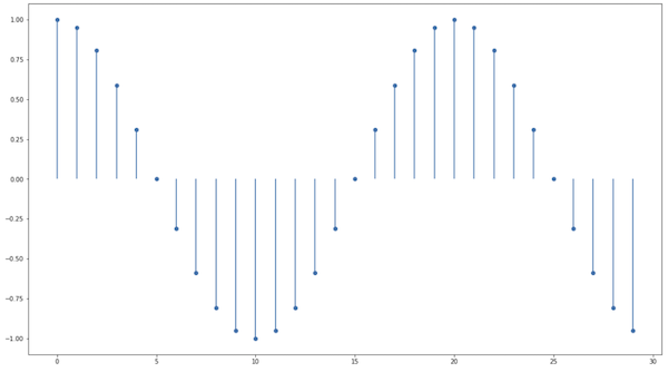
If we plot a line chart with $n$ as the x-axis and $cos (\omega n + \phi)$ the y-axis, we’ll see a points from a sinusoid. More familiar terms for $\phi$ is offset and for $\omega$ is step. A simple Python snipet to generate data points is:
ys = []
for t in range(N):
    ys.append(cos(t*step + offset))
The following graph displays samples using $\phi = \pi/2$ and $\omega = \pi/10$ and $N = 100$:
Complex values
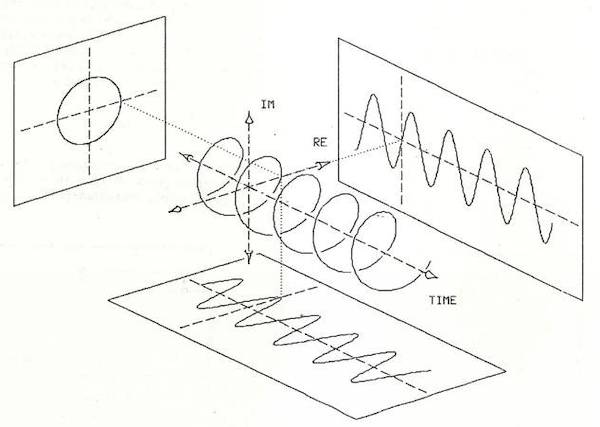
What does a complex number refer to in the real world? The insight provided by [1] is that $\mathbb{C}$ is just a convenient way to represent 2 real-valued entities. We could work with $\mathbb{R}^2$ all along, but the relationship between the two entities is such that complex numbers and all the machinery around it works neatly for signals.
We can visualize this in 3d, the 2 dimensions representing both components of the signal value and another the time:
Discrete Fourier Transform
Fourier Basis
We’ll now define a basis for the space $\mathbb{C}^N$ using the complex exponential signals described above.
Let $\vec{u}^{(k)}$ be a family (indexed by $k$) of finine complex exponential signals defined by:
\[u_t^{(k)} = e^{i \omega_k t} \qquad n = 0, \cdots, N-1\]We want each member of the family to have a different $\omega_k$. We’ll now see how to obtain $N$ such values.
The key point is that we will use this finite signal to generate a infinite periodic one via the periodic extension, in which case the $N$-th element should be the same as the $0$-th:
\[u_0^{(k)} = u_N^{(k)} = e^{i \omega_k 0} = 1\]We can then write:
\[u_N^{(k)} = (e^{i \omega_k})^N = 1\]This is the equation for root of unit, that is a complex number that yields 1 when raised to some power $N$.
For this case in particular, there are $N$ possible values satisfying this equation, namely:
\[e^{\frac{i 2\pi m}{N}} \qquad m = 0, \cdots, N-1\]So we can choose $\omega_k = \frac{2 \pi k}{N}$ and obtain $N$ distinct values. We can verify that for $t = N$,
\[e^{i \omega_k N} = e^{i 2 \pi k} = e^{i 2 \pi} = 1\]The signal $\vec{u}^{(k)}$ can now be re-written as
\[u_t^{(k)} = e^{i \frac{2 \pi k t}{N}} \qquad t, k = 0, \cdots, N-1\]The inner product of two elements $\vec{u}^{(n)}$ and $\vec{u}^{(m)}$ is
\[\langle \vec{u}^{(n)}, \vec{u}^{(m)} \rangle = \sum_{t=0}^{N-1} u^{(n)} \bar{u}^{(m)}\]Expanding their definition, and using the fact that the complex conjugate of $e^{ix}$ is $e^{-ix}$ we have:
\[= \sum_{t=0}^{N-1} e^{i (2 \pi n t)/N} e^{- i (2 \pi m t)/N}\] \[= \sum_{t=0}^{N-1} e^{i (2 \pi (n - m) t)/N}\]Let’s define $\alpha = e^{i (2 \pi (n - m))/N}$, so the sum above is
\[= \sum_{t=0}^{N-1} \alpha^t\]If $n = m$, then $\alpha = 1$, so the sum above is $N$. If $n \neq m$, we can use the close form of this geometric series:
\[= \frac{1 - \alpha^N}{1 - \alpha}\]We have that $\alpha^N = e^{i (2 \pi (n - m))} = 1$ and $\alpha \ne 1$ (since $0 < (2 \pi (n - m))/N < 2 \pi$), so the series above is 0. Summarizing:
\[\begin{equation} \langle \vec{u}^{(n)}, \vec{u}^{(m)} \rangle =\left\{ \begin{array}{@{}ll@{}} N, & \text{if}\ n = m \\ 0, & \text{otherwise} \end{array}\right. \end{equation}\]which proves that the vectors in the family are mutually orthogonal. The above also shows that the length of the vector is $\sqrt{N}$, since $\norm{\vec{u}^{(n)}}^2 = \langle \vec{u}^{(n)}, \vec{u}^{(n)} \rangle = N$. So if we want to make these orthonormal we just need to include the $\frac{1}{\sqrt{N}}$ factor in $\vec{u}^{(n)}$:
\[u_t^{(k)} = \frac{1}{\sqrt{N}} e^{i \frac{2 \pi k t}{N}} \quad t = 0, \cdots, N-1\]This shows $\vec{u}^{(k)}$ forms a basis for $C^N$, which is also know as Fourier basis.
DFT as a Change of Basis
Consider $\vec{x} \in \mathbb{C}^N$. It’s usually represented as $\vec{x} = (x_0, \cdots, x_{N-1})$ where $x_i$ is the coefficient of the linear combination of the canonical basis (i.e. $(1, \cdots, 0), (0, 1, \cdots, 0), \cdots (0, \cdots, 1)$) that generates $\vec{x}$.
We can also represent $\vec{x}$ as a linear combination of the Fourier basis, that is $\vec{u}^{(k)}$:
\[\vec{x} = \sum_{k=0}^{N-1} \lambda_k \vec{u}^{(k)}\]Recalling each element in $\vec{u}^{(k)}$ is defined as $u_t^{(k)} = \frac{1}{\sqrt{N}} e^{i \frac{2 \pi k t}{N}}$, $t = 0, \cdots, N-1$, we can also express a specific element in $x_t \in \vec{x}$:
\[(1) \quad x_t = \sum_{k=0}^{N-1} \lambda_k {u}^{(k)}_t = \frac{1}{\sqrt{N}} \sum_{k=0}^{N-1} \lambda_k e^{i \frac{2 \pi k t}{N}}\]This linear operation is invertible, so we can find $\lambda_k$ from $\vec{x}$:
\[(2) \quad \lambda_k = \frac{1}{\sqrt{N}} \sum_{t=0}^{N-1} x_t e^{- i \frac{2 \pi t k}{N}}\]Expression (2) should look familiar! It’s the discrete Fourier transform, while (1) is the inverse discrete Fourier transform. A more common form is to not include the factor $\frac{1}{\sqrt{N}}$ in $\vec{\lambda}$ by having
\[\quad \lambda'_k = \sum_{t=0}^{N-1} x_t e^{- i \frac{2 \pi t k}{N}}\]and then include it in (1):
\[(3) \quad x_t = \frac{1}{N} \sum_{k=0}^{N-1} \lambda'_k e^{i \frac{2 \pi k t}{N}}\]In signal processing, $\vec{x}$ is said to be in time domain, while $\vec{\lambda}$ in the frequency domain. In our vector space point of view, they can be seen as the representation of $\vec{x}$ in different basis, and the Fourier transform is a linear transformation that can be interpreted as a change of basis, mapping one set of coefficients into the other.
Discrete Fourier Series
The Discrete Fourier Series (DFS) generalizes the Discrete Fourier Transform (DFT) for signals $\widetilde{\vec{x}}$ which are infinite but periodic, that is, they have finite repeating pattern $\vec{x} \in \mathbb{C}^N$. The vector $\vec{u}^{(k)}$ is still the same except is now has infinite length:
\[u_t^{(k)} = \frac{1}{\sqrt{N}} e^{i \frac{2 \pi k t}{N}} \quad t \in Z\]Note that $\vec{u}^{(k)}$ is periodic.
The interesting part is we still only need $N$ vectors $\vec{u}^{(k)}$ to represent $\widetilde{\vec{x}}$, because even though it’s infinite in length, the pattern is finite. As an example to help with the intuition is the infinite periodic vector, consider $(1, 2, 3, 1, 2, 3, \cdots)$, with a finite pattern $(1, 2, 3)$. It can be defined as linear combination of only 3 infinite periodic vectors $(1, 0, 0, 1, 0, 0, \cdots)$, $(0, 1, 0, 0, 1, 0, \cdots)$ and $(0, 0, 1, 0, 0, 1, \cdots)$.
Equation (1) then becomes:
\[\widetilde{x}_t = \sum_{k=0}^{N-1} \lambda_k {u}^{(k)}_t = \frac{1}{\sqrt{N}} \sum_{k=0}^{N-1} \lambda_k e^{i \frac{2 \pi k t}{N}}\]Note that $\vec{\lambda}$ is of finite length $N$, but we can use periodic extension to turn into a infinite periodic vector $\widetilde{\vec{\lambda}}$ in which case the inverse applies:
\[\widetilde{\lambda}_t = \frac{1}{\sqrt{N}} \sum_{k=0}^{N-1} x_k e^{- i \frac{2 \pi k t}{N}}\]Discrete-Time Fourier Transform
The Discrete-Time Fourier Transform (DTFT) generalizes the Discrete Fourier Transform (DFT) for signals which are infinite and aperiodic.
We’ll see how to define the transform using the same basic ideas we did for DFT. Before that, let’s revisit the concept of Riemann sum.
Riemann Sum
The Riemman sum is a way to approximate the area under a continuous curve with discrete sum. This is basically the algorithm we use to compute the integral of a function in numerical analysis.
More formally, suppose we want to integrate $f(x)$ for $a \le x \le b$ ($x \in \mathbb{R}$). The idea is to define $N - 1$ discrete intervals for $x$, $[x_0, x_1], [x_1, x_2], \cdots, [x_{n-2}, x_{n-1}]$, where $x_0 = a$, $x_{n-1} = b$ and $\Delta_{x_i} = x_{i+1} - x_i$, then choose a representative $x_i^{*} \in [x_i, x_{i+1}]$ and sum their areas:
\[\int_{a}^{b} f(x) dx = \lim_{N \rightarrow \infty} \sum_{i=0}^{N-2} f(x^{*}_i) \Delta_{x_i}\]DTFT as a Limit of a DFT
We can now build some intuition by considering how the DFT looks like when $N \rightarrow \infty$.
As before, we’ll define $\omega_k = \frac{2 \pi k}{N}$ for $k = 0, \cdots, N-1$ and $\vec{u}^{(k)}$:
\[\vec{u}^{(k)}_t = e^{i \omega_k t} \quad t \in \mathbb{Z}\]And as before we can express any infinite signal $\vec{x}$ as a linear combination of $\vec{u}^{(k)}$ (3):
\[(4) \quad x_t = \frac{1}{N} \sum_{k = 0}^{N - 1} \lambda_k e^{i \omega_k t}\]We’ll massage (4) so that it’s defined in terms of $\omega_k$ and it looks like the right side of the Riemman sum.
Let’s define $\Delta_\omega$ as the distance between consecutive $\omega_k$, so $\Delta_{\omega_k} = \omega_{k + 1} - \omega_{k} = \frac{2\pi}{N}$. Note that $\Delta_{\omega_k}$ does not depend on the value of $k$, so we can also say $\Delta_{\omega_k} = \Delta_{\omega}$.
We can get rid of the $\frac{1}{\sqrt{N}}$ in (4) by defining it in terms of $\Delta_\omega$:
\[\quad x_t = \frac{\Delta_{\omega}}{2 \pi} \sum_{k = 0}^{N - 1} \lambda_k e^{i \omega_k t}\]We can push $\Delta_\omega$ inside the sum and add the index:
\[\quad x_t = \frac{1}{2 \pi} \sum_{k = 0}^{N - 1} \lambda_k e^{i \omega_k t} \Delta_{\omega_k}\]We can define $\lambda_k$ in terms of $\omega_k$ since $\vec{\lambda}$ is just a set of variables we’re defining and there’s a 1:1 mapping between $k$ and $\omega_k$, so we could just relabel $\lambda_k$ as $\lambda_{\omega_k}$. Let’s assume $\lambda$ is a function instead, so:
\[\quad x_t = \frac{1}{2 \pi} \sum_{k = 0}^{N - 1} \lambda(\omega_k) e^{i \omega_k t} \Delta_{\omega_k}\]Let’s also abstract $\lambda(\omega_k) e^{i \omega_k t}$ as a function of $\omega_k$, say, $f(\omega_k)$:
\[\quad x_t = \frac{1}{2 \pi} \sum_{k = 0}^{N - 1} f(\omega_k) \Delta_{\omega_k}\]This now looks like exactly as the format we wanted, observing that $\omega_k \in [\omega_{k+1}, \omega_k]$, $\omega_0 = 0$ and $\omega_{N-1} = 2 \pi$, we can express (4) as:
\[x_t = \frac{1}{2 \pi} \int_{0}^{2 \pi} f(\omega) d\omega\]We can “unwrap” $f$ and get:
\[(5) \quad x_t = \frac{1}{2 \pi} \int_{0}^{2 \pi} \lambda(\omega) e^{i \omega t} d\omega\]We can define the inverse of (5) to obtain $\lambda(\omega)$:
\[(6) \quad \lambda(\omega) = \sum_{t = 0}^{N-1} x_t e^{-i \omega t} \quad 0 \le \omega \le 2 \pi\]Another note on notation: $\lambda(\omega)$ is often denoted as $X(e^{i\omega})$ in signal processing [1] to make it obvious it’s a periodic function [1].
We can show that (6) is the inverse transform of (5).
Proof: We can verify this claim by replacing it in (5):
\[\frac{1}{2 \pi} \int_{0}^{2 \pi} (\sum_{j = 0}^{N-1} x_j e^{-i \omega j}) e^{i \omega t} d\omega\]Moving the second exponential into the sum and grouping them:
\[\frac{1}{2 \pi} \int_{0}^{2 \pi} \sum_{j = 0}^{N-1} x_j e^{i \omega (t - j)} d\omega\]We can also swap the sum and integral:
\[\frac{1}{2 \pi} \sum_{j = 0}^{N-1} x_j \int_{0}^{2 \pi} e^{i \omega (t - j)} d\omega\]Now if $t = j$, $\int_{0}^{2 \pi} e^{i \omega 0} = \int_{0}^{2 \pi} 1 = 2 \pi$. Otherwise, define $k = t - j$, $k \in \mathbb{Z}$. Then
\[\int_{0}^{2 \pi} e^{i \omega k} d\omega = \frac{1}{i k} e^{i \omega k} \bigg\rvert_{0}^{2 \pi} = \frac{1}{i k} (e^{i 2 \pi k} - e^{0}) = 0\]Since $e^{i 2 \pi k} = e^{0} = 1$, so the only index $j$ for which $e^{i \omega (t - j)}$ is non-zero is $j = t$, in which case it’s $2\pi$, which shows:
\[\frac{1}{2 \pi} \int_{0}^{2 \pi} (\sum_{j = 0}^{N-1} x_j e^{-i \omega j}) e^{i \omega t} d\omega = x_t\]QED
Convergence
For $\lambda(\omega)$ (6) to be defined, we need to show that its partial sums exist and are finite Let the $N$-th partial sum of (6) be $\lambda_N(\omega)$:
\[\lambda_N(\omega) = \sum_{t = 0}^{N-1} x_t e^{-i \omega t}\]If $\vec{x}$ is absolutely convergent, that is, there is $L$ such that
\[\sum_{t=0}^{N} \abs{x_t} = L, \qquad N \rightarrow \infty\]It’s possible to show that $\lambda_N(\omega)$ converges to $\lambda(\omega)$ uniformily, that is, for any arbitrary $\epsilon$,
\[|\lambda_N(\omega) - \lambda(\omega)| < \epsilon, \quad 0 \le \omega \le 2 \pi, N \rightarrow \infty\]And that $\lambda(\omega)$ is continuous.
On the other hand, if $\vec{x} \in \ell^2$ (i.e. it has finite energy), the above might not be the case. However it can be shown (the Riesz–Fischer theorem) that $\lambda_N(\omega)$ converges in regards to the $L^2[0, 2 \pi]$ norm, that is:
\[\int_{0}^{2 \pi} \norm{\lambda_N(\omega) - f(\omega)}^2 d\omega = 0\]when $N \rightarrow \infty$.
Another way to see this: if $\vec{x}$ is absolutely convergent, there’s a function that converges to $\lambda(\omega)$ exactly. If $\vec{x} \in \ell^2$, there’s a function that is not exactly like $\lambda(\omega)$, but is arbitrarily close when using $L^2[0, 2 \pi]$ to measure distance.
Summary
One way to quickly differentiate between DFT, DFS abd DTFT is based on the types of signals they’re defined for:
| Transform | Signal |
|---|---|
| DTF | Finite |
| DFS | Infinite, periodic |
| DTFT | Infinite, aperiodic |
Conclusion
In this post we butchered the notation from signal processing and handwaved rigour from the math side, so late apologies if this upset the reader.
Also in this post, we got some mathematical intuition behind Fourier transforms. I’ve known the signal processing interpretation of the Fourier transform as the decomposition of periodic signals into pure sinusoids, but the mathematical approach also adds more formalism and helps understanding some constraints such as why we would want signals with finite energy.
Related Posts
- Quantum Fourier Transform. We ran into Fourier transforms befire in the context of Quantum computing. At that time I relied on the transform formula without further insights on its origin.
