kuniga.me > NP-Incompleteness > KD-Tree

KD-Tree

31 Jul 2026

Jon Bentley is an American computer scientist, famously known for his book Programming Pearls. He also came up with the data structure called k-d tree while an undergrad at Stanford and published it in a paper titled Multidimensional Binary Search Trees Used for Associative Searching in 1975.

In this post we study the kd-tree data structure, how to construct and perform queries on it. Then we provide an implementation in Python.

Nearest Neighbors

The “kd” in kd-tree stands for k-dimensional tree. We can think of it as a generalization of a binary search. In one version of the binary search problem we are given an array and a query value $q$. We need to find the element in the array that is the closest to $q$. This is called nearest neighbors search.

The problem kd-tree solves is essentially the same but the values are points in a k-dimensional space instead of a scalar (1d). The variant we’re interested in is the static one, i.e. we don’t allow inserting, updating or removing points.

To solve the 1d case, we consider the points in the line and let $m$ be the median point. If $m < q$ then we can discard half of the points from the input, those having values less than $m$. If $m > q$, we do the same for the other half. If $m = q$, we found the closest point. This property allows us to find the nearest neighbor in 1d in $O(\log n)$ time by keeping the points sorted.

For the kd case, there’s no single ordering, so what can we do?

Partition

One way to see the search space of the 1d case is that of partitions organized as a binary search tree (BST). First we partition the points into 2: those with value less or equal than the median $m$, and those with value greater than $m$. Each partition has roughly the same number of points. We then subdivide each partition the same way, recursively, so we end up with a BST.

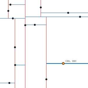
For the kd-tree we use the same idea but we “alternate” on which dimension to partition on. This is most intuitive for 2d: first we partition on the $x$ axis, i.e. we split the points by finding the median of the $x$ coordinate $x_m$ and have one partition contain all points with $x \le x_m$ and another the points with $x \gt x_m$.

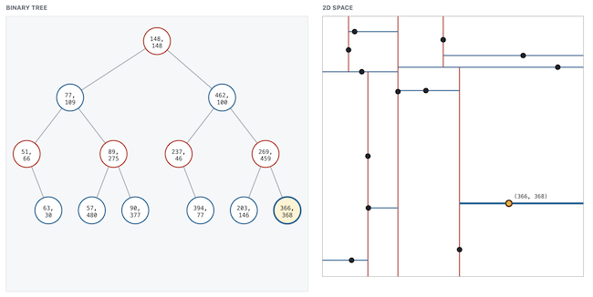
For the next level we partition on the $y$ axis instead. Geometrically each node in the 2nd level of the BST represents a quadrant containing roughly 1/4 of the points.

Searching

Unfortunately, for dimensions greater than 1, knowing which partition a query point $q$ belongs to does not allow us to discard the other half. Here’s a counter-example:

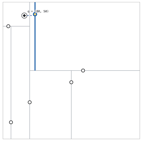
However, once we do find the partition of $q$, we do get an upper bound for the distance of the closest neighbor. This helps prune searches to the other partitions if there is not a lot of degeneracy.

So the idea of the algorithm is: traverse the BST to find the right partition and note the distance $d$ from $q$ to the point on that partition. As we backtrack, we ask “could this alternative branch contain the closest point?”.

We can quickly determine the lower bound between $q$ and any point of that branch by computing the distance between $q$ and the hyperplane (or line in the 2d case) which is $\abs{k_q - k_m}$ where $k$ is the dimension chosen for the partition and $k_m$ the median point. If this value is higher than $d$ we don’t need to keep searching. Otherwise we repeat the process there.

Once we reach the leaf on that subtree, we’ll potentially update $d$ and repeat the exact same process. In the worst case, we might end up visiting each leaf in this tree which would lead to a $O(n)$ complexity.

Implementation

We’ll implement a static, general dimension, kd-tree in Python. First we define some helper classes.

Data Structures

We start with Point, which is a thin wrapper on top of tuple, that implements some utility operators:

@dataclass(frozen=True)
class Point:
    data: tuple[int, ...]

    def __getitem__(self, dim: Dimension):
        return self.data[dim.v]

    def __len__(self) -> int:
        return len(self.data)

    def __abs__(self) -> float:
        return sqrt(sum(x*x for x in self.data))

    def __sub__(self, other: Point):
        sub = tuple(a-b for a,b in zip(self.data, other.data))
        return Point(sub)

Where Dimension is just a simple wrapper to carry around the max dimension so we can get the next dimension in modular fashion:

@dataclass(frozen=True)
class Dimension:
    n: int
    v: int = 0

    def next(self):
        next_v = (self.v + 1) % self.n
        return Dimension(self.n, next_v)

Since the kd-tree is a binary tree, the node is straightforward. We also add an is_leaf() to help with readability:

@dataclass
class KDNode:
    pivot: Point
    left: KDNode
    right: KDNode

    def is_leaf(self):
        return self.left is None and self.right is None

Finally we define a View class representing a sub-range, or a view, of a list. This is because we plan to avoid copying the array and instead work with sub-ranges of it:

@dataclass
class View:
    pts: list[Point]
    lo: int = 0
    hi: int | None = None

    def __post_init__(self):
        if self.hi is None:
            object.__setattr__(self, 'hi', len(self.pts) - 1)

    def range(self, lo, hi):
        return View(self.pts, lo, hi)

    def swap(self, i, j):
        self.pts[i], self.pts[j] = self.pts[j], self.pts[i]

    def __getitem__(self, i: int):
        return self.pts[i]

    def __setitem__(self, i: int, p: Point):
        self.pts[i] = p

Median

To construct the kd-tree we need to find the median point, i.e. a point such that half of the points in the set are smaller than it, and half are greater for a particular dimension. We can use the quick-select algorithm for this:

• Choose a random element from the array. Call it pivot
• Rearrange the array so that all elements smaller than pivot appear before it and all elements greater than it appear after.
• After this, if pivot is towards the beginning of the array, repeat for the right side of the array. If towards the end, repeat for the left side. The goal is to eventually have pivot appear at the middle of the array.

The partition() function below implements the second bullet point:

def partition(pts: View, p: int, dim: Dimension) -> int:
    """
    Lomuto partition. Rearrange pts[lo:hi] so that
    if i < p, then pts[i][dim] <= pts[p][dim]
    if i > p, then pts[i][dim] > pts[p][dim]
    """
    lo, hi = pts.lo, pts.hi
    pivot = pts[p]
    pts.swap(p, hi)
    store = lo

    for i in range(lo, hi):
        if pts[i][dim] <= pivot[dim]:
            pts.swap(store, i)
            store += 1

    pts.swap(store, hi)
    return store

The first and third points are implemented by the outer function:

def median_index(pts: View, dim: Dimension) -> int:
    lo, hi = pts.lo, pts.hi
    k = lo + (hi - lo) // 2
    while True:
        if lo == hi:
            return lo
        p = partition(pts.range(lo, hi), random.randint(lo, hi), dim)
        if p == k:
            return p
        elif p > k:
            hi = p - 1
        else:
            lo = p + 1

It’s possible to show this algorithm is $O(n)$ on average but $O(n^2)$ in the worst case.

Building

Open the interactive applet that builds a kd-tree.

Once we have the function to find the median, building the kd-tree is very simple:

def build_kd_tree(pts, dim):
    if pts.lo > pts.hi:
        return None

    mi = median_index(pts, dim)

    left = build_kd_tree(pts.range(pts.lo, mi - 1), dim.next())
    right = build_kd_tree(pts.range(mi + 1, pts.hi), dim.next())

    return KDNode(pivot=pts[mi], left=left, right=right)

Searching

Open the interactive nearest-neighbor search.

Search is relatively simple too, when traversing a node:

• Check if the current pivot is the closest point.
• Recurse on the query point’s partition.
• If the lower bound from the other partition is smaller than what we have so far, recurse on the other partition as well.

def query_kd_tree(node, q, dim, ub = inf):
    if not node:
        return None

    p = node.pivot

    if node.is_leaf():
        return p

    if q[dim] <= p[dim]:
        main = node.left
        other = node.right
    else:
        main = node.right
        other = node.left

    c = None

    # pivot is a candidate
    if dist(q, p) < ub:
        c = p
        ub = dist(q, p)

    # main branch
    c1 = query_kd_tree(main, q, dim.next(), ub)
    if dist(q, c1) < ub:
        c = c1
        ub = dist(q, c1)

    # minimum distance we can expect to find
    # on the other branch
    lb = abs(q[dim] - p[dim])
    if lb < ub:
        c2 = query_kd_tree(other, q, dim.next(), ub)
        if dist(q, c2) < ub:
            c = c2

    return c

In the best case the search behaves like binary search and it takes only $O(\log n)$ operations but in degenerate cases it can be $O(n)$ (i.e. all nodes of the tree need to be searched).

The full code is on Github.

Conclusion

Kd-tree is on my list of data structures or algorithms I had heard of, possibly used some existing implementation, but never took the time to study in detail. Another recent example is the Delaunay Triangulation.

One thing I skipped for this post is any theoretical analysis that shows how kd-trees perform on average.

The JavaScript applet was vibe-coded using Codex, which one-shot it (after finding a bug in my implementation) in less than 5 minutes, with this prompt verbatim:

I want to build a JavaScript self-contained app that shows how the kd-tree algoritm works. I’m going to use this implementation: /Users/kunigami/workspace/python/kd-tree/kd-tree.py . The idea: use svg to draw a 512 x 512 box, generate 13 random points. It should render the dividing line from the pivot. On the left, render a binary tree. Inside the node show the pivot point. Ok? We want to do this interactive, so we should have a parameter step. the rendering should go only up to step N while doing a pre-order ‘traversal’. Then we add buttons prev / next which increment N and re-render. Feasible?

This was provided more or less on the spot: you can see I added details after such as the buttons, so it wasn’t a well thought out prompt. I was astonished by the result. I have been using Claude Code to generate code and sometimes it does generate entire code features for me, but maybe because this one was visual, I felt more impressed!

I’m pretty sure there are many such applets out there from which the model can learn, so it probably helped in it being so successful.

It would have taken me hours to implement this and I wouldn’t have found it worth spending the extra time. With AI I can not only enrich my posts with these visualizations but build these while studying to better understand things.

It also built the search version of it in one shot. I need to raise my expectations for what LLMs can accomplish. In Delaunay Triangulation I said:

It did cross my mind to write a JavaScript-based on for the Bowyer-Watson algorithm, especially if Claude can do most of the implementation, but it would still take some work to test, polish and read the code, so I decided to pass.

Related Posts

Finding the median of a set of points efficiently is an interesting problem. T-Digest in Python tackles this statistical problem from a different angle: how to compute the P50 (and other percentiles) online, i.e. without storing all points explicitly.

Binary search trees, such as the red-black tree, implement the 1d version of the kd-tree but allow for efficient insertion and removal. In Consistent Hashing we use Rust’s implementation of a red-black tree to efficiently search the closest server of a given key in the “ring”.

Skip Lists is a probabilistic alternative to binary search trees for range search. A natural question is: can skip lists be generalized to k dimensions? Eppstein et al. have papers on those: The Skip Quadtree and Skip-webs.

Another multi-dimensional probabilistic structure for nearest neighbor search is called Hierarchical Navigable Small World, which is apparently very popular for vector search, an important aspect of modern ML.

Source code | RSS feed | Tags: computational geometry