kuniga.me > NP-Incompleteness > T-Digest in Python

T-Digest in Python

29 Nov 2021

T-Digest is a structure that can determine the percentile of a collection of values using very low memory without sacrificing too much accuracy. It was created by Ted Dunning and Otmar Ertl [1].

In this post we’ll explore the problem of determining percentiles, provide some naive solutions and then cover the t-digest to understand how it solves the problem more effectively.

Definitions

Values and Elements

Before we start, it’s important to clarify the subtle difference between what we’ll call an element vs its value. Two distinct elements can have the same value, so in the list [1, 10, 10, 3], the second and third elements have the same value.

In Python terms, an element is an instance while its value is a scalar:

@dataclass
class Integer:
    self.value: int

a = Integer(10)
b = Integer(10)

print(a == b) # False
print(a.value == b.value) # True

In this post, we’ll be pedantic about elements and values in order to make things less ambiguous.

Quantiles and Quantiles Indices

Suppose we’re given a sorted list of elements $\vec{x} = x_0 \le x_1 \le \cdots \le x_{n-1}$, $x_i \in \mathbb{R}$.

The median of this list is the value $M$ such that about half of the elements have values $\le M$ and the other half have values that are $\ge M$.

If $n$ is odd, since the list is sorted, the middle index contains the median, that is $M = x_m$ where $m = (n + 1) / 2$. If $n$ is odd, then we take the average of the two central elements, $M = (x_m + x_{m+1})/2$, where $m = n / 2$. Note that the median is a value that does not necessarily correspond to any of the elements.

We can generalize this idea. Instead of finding a value that “splits” the sorted list in halves, how about 1/3 and 2/3 split, or 9/10 and 1/10 split? This generalization is called a quantile.

Consider a real valued $0 \le \theta \le 1$. Let’s define $\theta$-quantile $q_{\theta}$ as the value such that $\theta \cdot n$ of the elements in the list are less or equal than $q_{\theta}$. We’ll call $\theta$ the quantile index of $q_{\theta}$. The median is thus $q_{1/2}$.

Quantiles vs. Percentiles

If the range $\theta$ is given as a number between 0 and 100 instead of 0 and 1, the corresponding value is called percentile and is often denoted by $p_{\theta}$, so for example $q_{0.75} = p_{75}$.

In this post we’ll only use quantiles to avoid working with multiple definitions.

Motivation

The quantile problem could be stated as: given a collection of values $x_0, x_1, \cdots, x_{n-1}$ (not necessarily sorted) and a quantile index $\theta$, return the quantile $q_\theta$ of the collection.

A simple way to solve this is to sort the elements and return the element $x_i$ for $i = k n$. This algorithm uses $O(n)$ memory and runs in $O(n \log n)$ time.

Let’s now consider the online version of this problem. In this variant, our list is infinite (or very large) $x_0, x_1 \le \cdots$, and from time to time we’ll send queries asking for the quantile $q_{\theta}$. This is the problem t-digest aims to solve.

It’s clear we can’t store all elements for this problem. We need to store a simplified representation of the elements such that it doesn’t take too much space but also approximates the data reasonably well.

It’s helpful to attempt to solve this problem using simple ideas to understand what problems we run into.

Histograms

First let’s try representing our sorted list $\vec{x}$ as a histogram. One interesting way to see a histogram is as a partition of $\vec{x}$ into intervals, where each intervals is called a bin.

So for example, if we have numbers $0, \cdots, 100$, we can partition this into a histogram with 2 bins, $0, \cdots, 30$ and $31, \cdots, 100$ or one with 10 bins, $(0, \cdots 10)$, $(11, \cdots 20)$, etc. Note the bin sizes can be of different sizes and represent intervals of different lengths.

The number of bins $m$ are usually much smaller than the number of elements $n$, and we only store a summary (or digest) of the elements in each bin, not an explicit list of elements. Thus we can reduce the memory footprint by representing elements as histograms.

In our case, the digest we’ll keep for each bin is simply the average of the elements in it and their count:

@dataclass
class Bin:
     avg: float
     size: int

Histogram With Interval-Lengths

In this version bins will represent intervals of same length, but may have different number of elements.

Let $x_{min}$ and $x_{max}$ be the minimum and maximum elements in $\vec{x}$, respectively. The index $j$ of the bin a value $x_i$ will belong is:

We can then assume all values in a given bin equals the average and from that it’s possible to compute the quantile $q_\theta$.

For example, suppose we used $m = 10$ and want to compute $q_{0.75}$. We know how many items there $n$ are in total and in each bin. To compute $q_{0.75}$ we need find the the $(0.75) \cdot n$-th item, which we can do via a simple scan of the bins.

Let’s suppose we find such element at bin $b^*$. The $q_{0.75}$ would then be the average of that bin. This could be very inaccurate if there’s a lot of variance inside the bin. For example, say that the bin contained the elements 100, 200, 300, and the $q_{0.75}$ was actually the element 300, but we’d report 200 since it’s the average of the bin.

Interpolation. For the example above, we know that the the $q_{0.75}$ is the last element at bin $b^{*}$ but we don’t know its true value. However, we can assume it’s also close in value to the elements in the next bin, $b^* + 1$, which perhaps has average 500 and thus we could do some linear combination between 200 and 500 to get some value closer to 300.

We’ll make the idea behind interpolation more precise but this should give a good idea on why interpolation is important.

The biggest problem with this approach is that we don’t know the maximum and minimum upfront. We would have to assume very large values to be safe, but then bins at the extremities would be unutilized and most of the elements would be concentrated in the middle bins.

In a degenerated case, all elements would fall under a single bin and every quantile would correspond to the average. In other words, we assumed the distribution of the elements is uniform.

Dynamic Range. We could make the bin ranges dynamic as we get new data, by keeping track of the minimum and maximum seen so far and redistribute the elements as min/max updates. The problem is that once we put an element on a bin we discard its value and replace by the average. We could use interpolation to approximate the values inside a bin but it seems that estimation errors would compound on each redistribution.

Histogram With Uniformly Sized Bins

So fixing the bin range is impractical due to the difficulty in estimating the minimum and maximum value. What if we fix the bin size, that is, limit the bin size to a fraction of the total size?

Each bin size would have size limited by $\lceil \frac{kn}{m} \rceil$, where $k$ is a small factor. As new elements come in we choose, from the bins that have space left, the ones whose average is the closest to the element.

If $k$ is too small, say 1, then most of the bins will be full at a given time, so there will be very few candidates to choose from, and adding elements will be almost like a Round-robin scheduling.

If $k$ is too large then we can choose from any bin at any time. Assuming some initial distribution of elements in the bins, adding elements will be like a k-means clustering, and the distribution will be strongly coupled with the initial distribution, which will be inaccurate if the stream of values is not ergodic (i.e. the overall distribution of values is consistent over time).

Having tested the water with some simple solutions, we should have a better sense of the problems with them and what needs to be addressed.

T-Digest

The t-digest is also a histogram, with the following high-level traits:

• The bin sizes are non-uniform. From [1]:

One key idea of the t-digest is that the size of each bin is chosen so that it is small enough to get accurate quantile estimates by interpolation, but large enough so that we don’t wind up with too many bins. Importantly, we force bins near both ends to be small while allowing sub-sequences in middle to be larger in order to get fairly constant relative accuracy.

• The number of bins can vary throughout the execution (but they’re bounded because merge operations reduce their size when they grow to too many)
• They might allow looser ordering between elements, so given $x > y$, $x$ might be placed in a lower bin than $y$ as long as $x$ is not much larger than $y$. From [1] again:

The other key idea is that there are practical algorithms that allow us to build t-digests incrementally, and although the result may not quite be strongly ordered, it will be close enough to be very useful

We’ll describe these properties in more details in the next sections. We’ll also provide Python implementations of the concepts as we discuss them.

Bin as Quantile Index Range

In the t-digest, it’s helpful to see a bin as representing a quantile index range. Another way to see this is that a bin represents an index range in a sorted vector, and a quantile is just a normalized version of those indexes.

For example, if we have a sorted list elements $\vec{x} = x_0, \cdots, x_{999}$, the element $x_{17}$ corresponds to the quantile index 17/1000. Thus a bin representing the indices range [17, 83] also represents the quantile index range [17/1000, 83/1000].

Bin Sizes & The Potential Function

To compute the bin size, the t-digest relies on a potential function $\pi(\theta)$, which is a function of the quantile index $\theta$ and it should be monotonically increasing.

The constraint is that the quantiles index range represented in a single bin cannot differ too much in their potential value. More formally, let $\ell$ be the lowest quantile in a given bin $b$ and $h$ the largest. We define $\sigma(b) = \pi(h) - \pi(\ell)$ as the potential difference of the bin $b$.

In a t-digest bins must satisfy:

Not a cumulative distribution. On reading of [1], my first interpretation was that $\pi(\theta)$ is a cumulative distribution function of $\theta$, but it’s not the case. In fact, a cumulative sum $f(\theta)$ would not give us much information, since by definition $\theta$ is just a normalized cumulative sum, that is, $f(\theta) = n \theta$, where $n$ is the total number of elements.

Bin mapping function? Wouldn’t it be more intuitive to define a function that maps a quantile index to a bin? Say $f(\theta)$ returns a value from 0 to 1 and the bin a quantile belongs to is given by $\lfloor \theta m \rfloor$ where $m$ is the number of bins? One example where this would be really bad is when the elements being inserted are decreasing. Each element being inserted would always map to the 0-th quantile and would go to the first bin. The potential function would prevent this because putting all elements in the same bin would violate (1).

The authors in [1] propose the following potential function:

Where the constant $\delta$ serves as the scaling factor and controls the number of bins. The number of bins in the t-digest will be between $\lfloor \frac{\delta}{2} \rfloor$ and $\lceil \delta \rceil$.

A simple Python implementation is given below:

from math import pi, asin
def get_potential(qid: float, delta=10):
    return delta * asin(2*qid - 1) / (2*pi)

The graph below from [1] shows how the function $\pi$ (called $k$ in the paper) varies over $\theta$ (called $q$ in the paper):

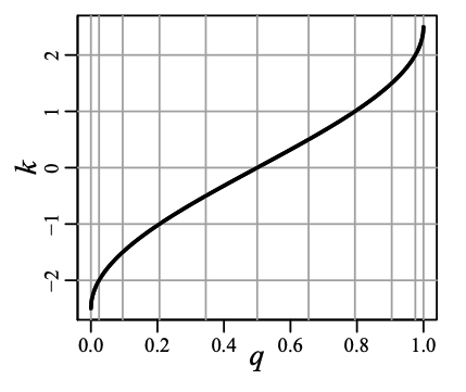
We can see that $\abs{f(\theta)}$ is symmetric around $\theta = 0.5$ and it varies a lot at the extremes. Big variance in the potential function implies smaller bin sizes because of the constraint (1).

Merging Two Bins

Let $\sigma(b_i)$ be the potential difference of a bin $b_i$. The potential difference of the combined bin $b_i$ and $b_{i+1}$ is given by:

Two adjacent bins can be merged if their combined potential difference does not violate constraint (1). Thus, $b_i$ and $b_{i+1}$ can be merged if:

To create a new bin corresponding to the union of two bins, we need to retrieve their total weight so we can compute the new average:

def merge_bins(x: Bin, y: Bin) -> Bin:
    weight = x.avg * x.size + y.avg * y.size
    size = x.size + y.size
    return Bin(avg=weight/size, size=size)

Combining T-Digests

Suppose we’re given two lists of bins corresponding to two t-digests, with $n_1$ and $n_2$ elements, respectively. We can merge them into one and compress the bins.

def combine(t1: TDigest, t2: TDigest) -> TDigest:
    merged_bins = merge_bins(t1.bins, t2.bins)
    return compress(merged_bins)

Merging Two Lists of Bins

First we combine the bins into a single list and sort them by their mean. Since the each list is already sorted by their mean, we can do a simple merge sort like the Python code below:

def merge_bins(xs: List[Bin], ys: List[Bin]) -> List[Bin]:
    merged = []
    i, j = 0, 0
    while i < len(xs) and j < len(ys):
        if xs[i].avg <= ys[j].avg:
            merged.append(xs[i])
            i += 1
        else:
            merged.append(ys[j])
            j +=  1

    while i < len(xs):
        merged.append(xs[i])
        i +=  1

    while j < len(ys):
        merged.append(ys[j])
        j +=  1

    return merged

Compressing a List of Bins

We can now compress the bins in a greedy fashion. Let $\vec{b}$ represent the list of merged bins and let $\vec{b’}$ the result of compressing $\vec{b}$. At any given iteration $i$, we’ll try to merge bin $b_i$ into the current compressed bin $\vec{b’_k}$.

We can combine $b_i$ into $b_k’$ if $\sigma(b_k’) + \sigma(b_{i}) \le 1$ as mentioned in (3). If that’s not the case, we start a new merged bin $b’_{k + 1} = b_i$.

A Python implementation follows:

def compress(xs: List[Bin]) -> List[Bin]:
    if len(xs) == 0:
        return xs

    n = sum([x.size for x in xs])
    ys = [xs[0]]
    # lowest potential of the current
    # merged bin ys[-1]
    min_potential = get_potential(0)
    total = xs[0].size

    for i in range(1, len(xs)):
        x = xs[i]
        next_qid = 1.0 * (total + x.size) / n

        if get_potential(next_qid) - min_potential <= 1:
            ys[-1] = ys[-1] + x
        else:
            ys.append(x)
            min_potential = get_potential(1.0 * total / n)

        total += x.size

    return ys

One problem with this implementation is that it calls the function potential() $O(n)$ times where $n$ is the size of xs. The authors in [1] provide an optimized implementation that involves also using the inverse of the potential function, but it’s only called $O(k)$ times, where $k$ is the size of the compressed bins ys.

Since $n >\,> k$ and asin() is expensive to compute, the optimization can lead to significant speedups. We’ll now discuss the idea behind the optimized implementation.

Compressing T-Digests Optimized

Suppose the lowest quantile index for the current bin $b_k’$ being merged is $\ell$. We can compute $h$ by first finding the potential for $\ell$, $\pi(\ell)$. We know the maximum potential difference is 1, so the maximum potential of a quantile index should be $\pi(\ell) + 1$.

We can then use the inverse of $\pi()$ to find the quantile index given a potential, which should be possible since $\pi()$ is bijective. Thus,

We can combine the bin $b_i$ into $b_k’$ if the resulting maximum quantile index is less than $h$. We know how many elements we’ve seen so far (which is the sum of the elements in bins already processed, including the bin $b_k’$ being merged onto), which we’ll call $s_k$. So the maximum quantile will be given by:

If $\theta’ \le h$ we can merge $b_i$ into $b_k’$. Otherwise, we start a new merged bin $b’_{k + 1} = b_i$.

Inverting (2) is straightforward. We define $p$ as the potential $\pi(\theta)$ and re-write $p$ as a function of $\theta$:

In Python:

def get_inv_potential(p, delta=10):
    return (sin(p*2*pi / delta) + 1) / 2

The optimized version of compress() is quite similar:

def max_quantile_idx(qid: float) -> float:
    return get_inv_potential(get_potential(qid) + 1)

def compress_fast(xs: list[Bin]) -> list[Bin]:
    n = sum([x.size for x in xs])
    ys = [xs[0]]

    total = xs[0].size
    max_qid = max_quantile_idx(0)

    for i in range(1, len(xs)):
        x = xs[i]
        next_qid = 1.0 * (total + x.size) / n

        if next_qid <= max_qid:
            ys[-1] = merge_bin(ys[-1], x)
        else:
            ys.append(x)
            max_qid = max_quantile_idx(1.0 * total / n)

        total += x.size

    return ys

We can now see we call potential() and its inverse $O(k)$ times.

Inserting Elements

We can use the merge algorithm to insert elements in batch. We buffer the inputs into an array until it reaches a certain size.

Noting that a single element is a trivial bin with size 1 and average equal to the element’s value, we conclude that if the buffered elements are sorted, they form a t-digest, which can be merged into the existing t-digest.

The Python implementation using functions defined above is simple:

def insert_batch(ts: list[Bin], xs: list[float]) -> list[Bin]:
    ts2 = [Bin(avg=x, size=1) for x in xs]
    return merge(ts, ts2)

Querying

Once we have a t-digest, we should be able to, given a quantile index $\theta$, determine the approximate quantile of the current set.

One approach is to just find the bin to which the quantile index belongs to and return its average. However, if the quantile index is closer to the high end of the bin, we should also take into account the “influence” from the next bin. Similarly, if it’s closer to the low end of the bin, we leverage the previous bin. We can use interpolation as we discussed in the Histogram With Interval-Lengths section.

Given a bin $b$ with quantile index range $(\ell, h)$, the middle quantile index can be computed as $\bar \theta = (\ell + h)/2$.

There are 3 possible locations where the quantile index $\theta$ can be in regards to the middle quantile index:

• To the left of the first bin $b_0$:

• Between two bins $b_i$ and $b_{i+1}$:

• To the right of the last bin $b_m$:

In the first and third cases, we just assume the quantile is the bin’s average. On the second case, we can assume the quantile varies linearly between $\overline{\theta_{i}}$ and $\overline{\theta_{i + 1}}$. We compute the “slope” of this linear function as:

The quantile is then:

By calling $\Delta_{\theta} = \overline{\theta_{i + 1}} - \overline{\theta_{i}}$, we can re-arrange the terms as:

If we define $\lambda = (\theta - \overline{\theta_{i}})/\Delta_{\theta}$, it’s possible to obtain:

def get_quantile(t: TDigest, qid: float) -> float:
    bins = t.bins

    # if the elements were sorted, idx would represent the
    # index in the array corresponding to the quantile index qid
    idx = qid * get_elements_count()

    max_idx = bins[0].size / 2

    # idx is on the first half of the first bin
    if idx < max_idx:
        return bins[0].avg

    for i in range(len(bins) - 1):
        b = bins[i]
        b_next = bins[i + 1]

        interval_length = (b.size + b_next.size) / 2
        # target index is in between b and b_next. interpolate
        if idx <= max_idx + interval_length:
            lambda = (idx - max_idx) / interval_length
            return b.avg * (1 - lambda) + b_next.avg * lambda

        max_idx += interval_length

    # idx is on the second half of the last bin
    return bins[-1].avg

Experiments

All the experiments below use 10,000 values and $\delta = 10$ in the potential function (2).

Experiment 1. Elements sampled from a Gaussian distribution:

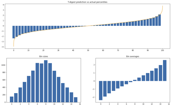
We can see it matches the actual distribution pretty well except on the extremes. The maximum value of the sample is around 4 while the maximum possible prediction (which is the average of the last bin) is 2.6.

Experiment 2. House prices from a Kaggle dataset:

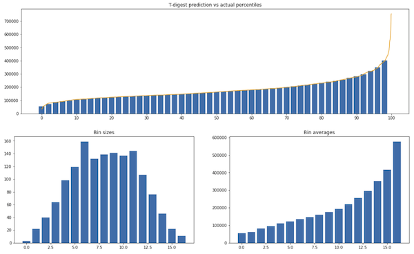
Similarly to the previous experiment, only the extremes are misrepresented. The maximum value of the data is 755k, while the maximum possible prediction is 577k.

Experiment 3. Sorted values from $x^2$:

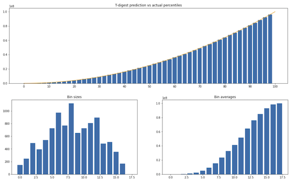
t-digest works well with sorted insertions, which is a case where the naive mapping of quantiles to bins would do poorly.

Source

The full implementation is on my Github as a Jupyter notebook. There’s a more efficient implementation in CamDavidsonPilon/tdigest, where insertions are $O(\log m)$.

Conclusion

I had no idea about how t-digest worked and am happy with my current understanding. T-Digest is an approximate data structure which trades-off accuracy for low memory footprint. The implementation is relatively simple, but the theory behind less so.

One way I see t-digests is as a histogram with dynamic bin sizes. The bin sizes fit a pre-determined distribution (given by potential function), which is similar to a Gaussian distribution (concentrated around the middle, sparse on the extremities).

One particular difficulty while reading the t-digest’s original paper [1] is that they don’t seem to have a name for the quantile index, sometimes even overloading it to be the quantile itself. I found easier to understand by having a special term for is, so I decided to give it a name.

It was very helpful to look up the implementation of CamDavidsonPilon/tdigest, since the paper didn’t make it super obvious how to implement interpolation while it was clear from the implementation. The funny thing is that I actually found a bug in their implementation and my fix was merged!

Related Posts

Huffman Coding and Linear Predictive Coding in Python are two other posts about compression. Huffman is lossless, while LPC is lossy like the t-digest.

The t-digest paper [1] mentions a result from information theory by Munro and Paterson, stating that computing any particular quantile exactly in $p$ passes through the data requires $\Omega(n^{1/p})$ memory. It makes me wonder about theoretical results around the tradeoffs of accuracy and memory footprint.

Bloom Filters and HyperLogLog in Rust describe two other data structures that fall under the same category of approximate data structures with very low memory footprint. Bloom filters are used for approximate membership test and HyperLogLog for approximate count of distinct values. Both are also relatively straightforward to implement but their guarantees are non-trivial.

References

• [1] Computing Extremely Accurate Quantiles Using t-Digests
• [2] Percentile and Quantile Estimation of Big Data: The t-Digest
• [3] Github: CamDavidsonPilon/tdigest

Source code | RSS feed | Tags: data structures, probabilistic algorithms, statistics, python