kuniga.me > NP-Incompleteness > Delaunay Triangulation
Delaunay Triangulation
20 Jun 2026
Boris Nikolayevich Delaunay was a Russian mathematician (1890 – 1980), who is best known for inventing the Delaunay triangulation.
Boris was the descendant of a French army officer de Launay, who was captured in Russia during Napoleon’s failed attempt to invade Russia. After his release, De Launay stayed back in Russia and married into a noble Russian family.
In this post we’ll study the Delaunay triangulation and the Bowyer–Watson algorithm for finding a Delaunay triangulation in $O(n^2)$.
Triangulation
Let $P$ be a set of points in the plane and such that no 3 points are collinear. An edge is a segment of line connecting a pair of points. Two edges intersect if their corresponding segments intersect. A triangulation can be defined as any maximal set of edges that do not intersect.
One way of getting an intuition about this property is to imagine we’re constructing a triangulation randomly: choose any pair of points that are not yet connected and try adding an edge. If this edge doesn’t intersect any existing edge, keep it, else choose the next pair. If we cannot find any edge to add, we have a maximal set and thus a triangulation.
A more visual way to define a triangulation is that all the faces (a bounded region not containing any points except its vertices) are triangles and the outer face (external edges) is the convex hull of $P$.
The advantage of this second definition is that it generalizes to higher dimensions. In 3D a triangulation is a set of edges such that all faces are tetrahedra and the outer face is the 3D convex hull of $P$.
Properties
Lemma 1. Let $P$ be a set of $n$ points in 2D and $h$ the number of points in its convex hull. Then the number of edges in any triangulation is:
\[e = 3n - 3 - h\]This means that for any fixed set of points, since its convex hull is unique, the number of edges is the same for any triangulation and also $O(n)$.
Delaunay Triangulation
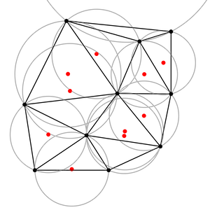
The intuition about the Delaunay triangulation is that it avoids “skinny” triangles. It achieves that by requiring that for every triangle in the triangulation its circumcircle contains no other points in its interior. When a triangle is skinny, their vertices are closer to be collinear and the circumcircle blows out, increasing the likelihood of including other vertices.
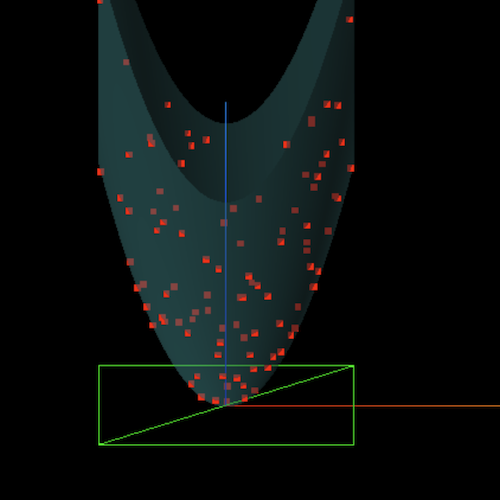
It’s not obvious why it’s always possible to find a triangulation with this property. To prove that, we first need to introduce a technique called lifting. It consists in mapping each 2D point $(x, y)$ to a 3D one $(x, y, x^2 + y^2)$. Geometrically this is lifting the points onto the surface of the paraboloid $z = x^2 + y^2$. We denote by $p_i$ a point in the original set $P$ and by $p’_i$ the corresponding lifted point.
The first interesting observation is that circles map to planes in the lifted space.
Lemma 2. Let $p_1, p_2$ and $p_3$ be non-collinear points from $P$. They form a unique circle, which uniquely maps to a plane in the lifted space containing $p’_1$, $p’_2$ and $p’_3$.
Now suppose a point lies inside the circle induced by $p_1, p_2$ and $p_3$. What’s the relation with the corresponding plane in the lifted space?
Lemma 3. Let $C$ be the circle induced by $p_1, p_2$ and $p_3$. If a point $q$ lies inside $C$, it lies “below” the corresponding plane $P$ in the lifted space. If it is in $C$, it belongs to $P$ and if outside $C$ it lies “above” $P$.
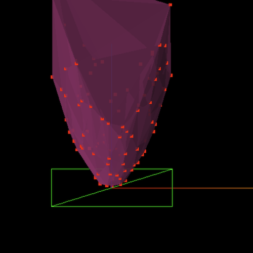
Now take the 3D convex hull of the lifted points, which will be a polyhedron with faces. Consider a face that is visible from below. It contains a set of points $p’_1, p’_2, \cdots p’_k$ (mostly $k=3$ but it’s possible to have more in degenerate cases). By definition these points are coplanar, and since the circle to plane mapping is unique, the corresponding points $p_1, p_2, \cdots p_k$ must be cocircular in the $xy$-plane.
We claim that such a circle contains no other point of $P$. If it did, by Lemma 3 it would map to a lifted point below the plane, which would then lie outside the convex hull, a contradiction. So this satisfies the constraint of the Delaunay triangulation. However, it’s possible that $k \gt 3$ but in that case we can triangulate the corresponding polygon in any way we want since for any 3 points we’ll obtain the same circle which will still not contain the other inside.
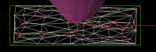
By construction we can guarantee every lifted point belongs to at least one face of the convex hull that is visible from below. So if we project each face that is visible from below onto the $xy$-plane and perform triangulation of the degenerate cases, we’ll obtain a Delaunay triangulation!
This proves not only that a Delaunay triangulation always exists but also provides an algorithm to find one.
Corollary E. The Delaunay triangulation always exists for a set of non-collinear points.
It’s also possible to show that if there are no cocircular points in $P$, then every Delaunay triangulation maps to the convex hull of the lifted space and hence that it is unique.
The Bowyer–Watson Algorithm
The algorithm is conceptually simple. We start with an empty triangle that is big enough to contain all points in $P$. Suppose its vertices are $a, b, c$, then this triangle is the Delaunay triangulation for $a, b, c$.
Then we insert one point $p$ of $P$ at a time, removing and adding some edges such that the resulting triangulation is a Delaunay triangulation for the $a, b, c$ and all the points of $P$ added so far. At the end we remove $a, b, c$ and any edges connecting to them and we end up with a Delaunay triangulation for $P$.
A more precise implementation is the following:
def compute_delaunay(P):
    t0 = bounding_triangle(P)
    tris = [t0]
    for p in P:
        bad_tris = []
        good_tris = []
        for t in tris:
            if in_circumcircle(t, p):
                bad_tris.append(t)
            else:
                good_tris.append(t)
        boundary = edges_used_once(bad_tris)
        for (a, b) in boundary:
            good_tris.append((a, b, p))
        tris = good_tris

    a, b, c = t0
    tris = [
        t for t in tris if not has_any_vertex(t, [a, b, c])
    ]
    return tris
The complexity of this algorithm is $O(n^2)$ because of the 2 nested loops and the fact that the number of triangles in a triangulation is $O(n)$. But it’s possible to optimize the bad triangle search to $O(\log n)$, to obtain a sub-quadratic algorithm.
Lemma 4 handles the more difficult task of proving the algorithm is correct. The gist of the proof is to show that what the algorithm is doing is essentially constructing the 3D convex hull of the lifted space incrementally.
Lemma 4. The Bowyer–Watson algorithm finds the Delaunay triangulation of a set of non-collinear points $P$.
The first thing we observe is that `bad_tris` is never empty. That's because since `p` lies inside the bounding triangle and `tris` is a valid triangulation for it, it must lie inside one triangle `x, y, z`, so such a triangle is bad. Note that it can't lie on the edge because we're assuming no three points are collinear.
The point `p` we're adding is contained in the circumcircles of `bad_tris`. Using the lifting argument these triangles correspond to faces in the convex hull visible from below. Since `p` is inside their circles by Lemma 3 it lies "below" the supporting plane of those faces. This also means `p` is outside of the existing convex hull and we wish to extend it to include `p`.
If we were to shine light from `p`, it would illuminate all the faces from the bad triangles but not the good ones. A convex hull containing `p` then would not contain the illuminated faces. Due to convexity, the union of the bad faces forms a contiguous region. We can remove these faces and then connect the vertices of the hole with `p`. Since `p` is now coplanar with the vertices that were previously violating the Delaunay condition, this new triangulation is a Delaunay one. This process is essentially computing the 3D convex hull of the lifted points iteratively (i.e. an online algorithm).
Now we show the correctness of the last step. Removing a point from a convex hull only removes the faces adjacent to it. Since `a, b, c` are the outermost vertices, their removal won't affect faces involving only vertices of `P`, so the remaining faces visible from below are from the convex hull of `P` and is thus a Delaunay triangulation of `P`.
We can complete the implementation by defining the functions we used above, starting with bounding_triangle().
Bounding Triangle
Any sufficiently large triangle will do, but if we want to keep it relatively tight on the data, we can do:
def bounding_triangle(P):
    "right triangle guaranteed to strictly contain all points of P"
    xs = [x for x, _ in P]
    ys = [y for _, y in P]
    minx, maxx = min(xs), max(xs)
    miny, maxy = min(ys), max(ys)
    d = max(maxx - minx, maxy - miny, 1)
    a = (minx - d, miny - d)
    b = (maxx + 3 * d, miny - d)
    c = (minx - d, maxy + 3 * d)
    return (a, b, c)
Point inside circumcircle
We can use the lifting technique and instead of determining whether a point $p$ is inside the circumcircle of a triangle $a, b, c$ (which would require finding the circle equation and taking square roots), we check if it’s “below” the supporting plane of their corresponding lifted points.
Lemma 5. Let $a = (a_x, a_y), b = (b_x, b_y), c = (c_x, c_y)$ be vertices of a triangle oriented counter-clockwise. Then a point $p = (p_x, p_y)$ lies within the circumcircle of this triangle if:
\[\det \begin{pmatrix} a_x-p_x & a_y-p_y & a_z-p_z \\ b_x-p_x & b_y-p_y & b_z-p_z \\ c_x-p_x & c_y-p_y & c_z-p_z \end{pmatrix} \gt 0\]The code then consists of evaluating this determinant explicitly:
def orient(a, b, c) -> int:
    return (b[0] - a[0]) * (c[1] - a[1]) - (b[1] - a[1]) * (c[0] - a[0])

def in_circumcircle(t, p) -> bool:
    a, b, c = t
    # normalize to counterclockwise
    if orient(a, b, c) < 0:
        b, c = c, b
    ax, ay = a[0] - p[0], a[1] - p[1]
    bx, by = b[0] - p[0], b[1] - p[1]
    cx, cy = c[0] - p[0], c[1] - p[1]
    det = (
        (ax * ax + ay * ay) * (bx * cy - cx * by)
        - (bx * bx + by * by) * (ax * cy - cx * ay)
        + (cx * cx + cy * cy) * (ax * by - bx * ay)
    )
    return det > 0
Boundary
Finding the boundary is relatively easy. We just need to count the frequency of each edge and only keep those that only appear once:
def edge(p1, p2):
    "normalized edge"
    return (p1, p2) if p1 < p2 else (p2, p1)

def edge_freq(tris):
    freq = defaultdict(int)
    for (a, b, c) in tris:
        freq[edge(a, b)] += 1
        freq[edge(a, c)] += 1
        freq[edge(b, c)] += 1
    return freq

def edges_used_once(tris):
    freq = edge_freq(tris)
    uniq_edges = []
    for e, cnt in freq.items():
        if cnt == 1:
            uniq_edges.append(e)
    return uniq_edges
Has Vertices
The last function is the easiest, there’s not much to explain:
def has_any_vertex(t, vs):
    for v in vs:
        if v in t:
            return True
    return False
Validation
One way to test the correctness of our implementation is to check if the resulting triangulation is Delaunay. Which is applying the definition that no points in $P$ are in the circumcircle of a triangle in the triangulation.
def is_delaunay(P, tris):
    for p in P:
        for t in tris:
           if in_circumcircle(t, p):
            return False
    return True

tris = compute_delaunay(P)
assert is_delaunay(P, tris)
We can also check if some properties of the triangulation holds:
from scipy.spatial import ConvexHull

hull = ConvexHull(P)
h = len(hull.vertices)

e = len(edge_freq(tris))
n = len(P)

assert e == 3 * n - 3 - h
The full code is on Github.
Conclusion
I had a lot of fun studying the Delaunay triangulation and the implementation of the Bowyer-Watson algorithm. Computational geometry was my favorite theoretical computer science subject and I did my master’s in this area.
I took a graduate class in Computational geometry and I do recall hearing about Voronoi and Delaunay triangulation but don’t recall how deep the classes went on these topics. I’d be very sad if I actually studied the proofs and the algorithm before because it felt very novel to me. I think about this often.
We’ve seen the relationship between Delaunay and 3D convex hulls here. In the future I hope to connect them to Voronoi diagrams as well.
Related Posts
In On Lifetime I mention that I wrote Java applets for interactive computational geometry algorithms such as for polygon triangulation and finding the convex hull in 2D! It did cross my mind to write a JavaScript-based on for the Bowyer-Watson algorithm, especially if Claude can do most of the implementation, but it would still take some work to test, polish and read the code, so I decided to pass.
In the The Gauss-Lucas Theorem we also deal with convex hulls and I used the same Python library scipy.spatial.ConvexHull for validating the number of edges property.
