kuniga.me > NP-Incompleteness > [Paper] State Management In Apache Flink
[Paper] State Management In Apache Flink
18 Aug 2022
In this post we’ll discuss the paper State Management In Apache Flink: Consistent Stateful Distributed Stream Processing by Carbone et al. [1]. This paper goes over the details of how state is implemented in Flink, an open-source distributed stream processing system. Great emphasis is given on fault-tolerance and reconfiguration mechanisms using snapshots.
Flink Architecture Overview
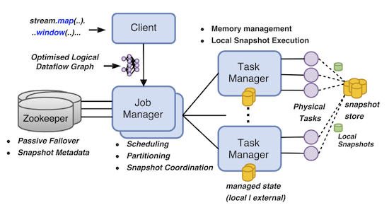
Flink has a programmatic API for specifying pipelines like FlumeJava [2] (in either Java, Python and Scala). The user writes the business logic using this API which gets converted into a logical graph.
This logical graph gets optimized on the client (e.g. operator fusion like in FlumeJava [2]) and sent to Flink’s runtime, where it gets converted to a physical graph composed of operators (e.g. source, mapper, reducer, sink). Each operator has one or more tasks that execute the actual work.
The system is composed of a set of machines, each running a task manager, which coordinates the tasks executing work in that host. There’s a central host that orchestrates the entire application, the job manager. Communication between task managers and the job manager happen via RPC.
To achieve high-availability with a centralized job manager, Flink keeps a set of stand-by replicas which can be promoted to leader in case of leader failures. The leader selection is achieved using Zookeeper [3].
Figure 1 shows a diagram with these components.
State
Managed State
We can divide state into two types based on scope: key and operator. The key scope state is per each key. For example, if we perform a group by key (say user ID) and then do an aggregation, the state storing the aggregated value is specific to a given key.
An operator scope state is a higher-level scope when it’s not specific to any task in particular. One example is the state needed to store the offsets when reading from Kafka. It pertains to the source operator as a whole, and is needed for checkpointing, i.e., upon recovery we want to resume reading from Kafka at a specific point in time.
State Partitioning
Keys are grouped into units called key groups. The number of key groups is fixed while the number of keys is application dependent.
Each group is the atomic in regards to a task assignment. This means that not only a task handles all keys from the group but upon reconfiguration (say adding new machines), the keys are re-assigned as a unit to another task.
This also makes key-state cheaper to access: keys from the same group can be stored sequentially/together so we reduce the lookups needed when the state is stored remotely.
There are more key groups than tasks, so a given task handles multiple key groups. The assignment is done contiguously to optimize read patterns (i.e. reduce seeks). So for example, if key groups are numbered $1$ to $K$, then each task gets the key groups from $\lceil i \frac{K}{T} \rceil$ to $\lfloor (i + 1) \frac{K}{T} \rfloor$ where $T$ is the total number of tasks.
Snapshots
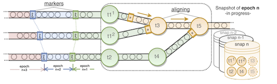
A data stream within Flink is conceptually divided in segments based on processing time (see [4] for terminology). More precisely each element belongs to a set which is identified by a timestamp and thus called epoch. This grouping is orthogonal to any application logic, including windowing.
The system interleaves epoch markers with the events so it gets propagated through the pipeline. Since the segmentation is based on processing time, streams processed in parallel belong to the same epoch. Figure 2 makes it much clearer.
Epochs are useful for the system to determine when to perform snapshots. Snapshots are taken at each task. When it observes an epoch marker $n$, it persists the current state adding to a centralized snapshot storage (distributed file system). When each task has snapshotted its epoch $n$, the system can complete the centralized snapshot for epoch $n$. If a failure happens, the system can restart the state from the complete snapshot with highest epoch.
It’s worth noting that a task doesn’t need to wait for another while taking partial snapshots: it’s possible a task has already created snapshot for say, epoch $n + 2$, while some tasks are still to snapshot epoch $n$.
To me, epoch sounds very similar to watermarks [4]. A watermark is a timestamp $w$ that says “I’ve seen all data with timestamps less than $w$”, whereas an epoch is a timestamp $e$ that says “I’ve snapshotted all data with timestamps less than $e$”.
Epoch Alignment
When two or more streams are merged like in $t3$ and $t5$ in Figure 2, tasks need to align the epoch markers of these streams. They can stop processing inputs from the stream that is ahead until the others catch up.
We can assume each stream implements an interface Stream containing block() which makes the stream stop reading data from the source and unblock() which reverts the block. The stream also implements a queue-like interface, with send(event) which causes some data/marker to be added to the end of the stream and get() to read an event at the front.
Algorithm 1 in Python below describes the alignment in each task, assuming input_streams and output_streams are of type List[Stream]:
blocked = set()
marker = None
while True:
  for input_stream in input_streams:
    event = input_stream.get()
    if input_stream not in blocked and isinstance(event, EpochMarker):
      input_stream.block()
      blocked.add(input_stream)
      marker = event

    if blocked == input_streams:
      for each output_stream in output_streams:
        output.send(marker)

      trigger_snapshot()

      for each input_stream in blocked:
        input_stream.unblock()
blocked = set()Cyclic Graphs
Flink supports cyclics graphs for interactive computations, so snapshotting must support this topology.
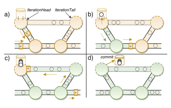
To implement this, Flink adds two special tasks, IterationHead and IterationTail which are co-located and share memory. For example, given a cycle $A \rightarrow B \rightarrow A$ the special tasks ($t$ for tail and $h$ for head) are inserted somewhere in the cycle like $A \rightarrow B \rightarrow t \rightarrow h \rightarrow A$.
Once the header task $h$ processes the epoch mark $n-1$, it will emit an epoch mark $n$. Once the tail task $t$ receives that epoch mark, it can be sure $h$ has processed all the events prior to the epoch mark $n$.
Figure 3. illustrates this idea. Notice that upstream tasks will also send their own epoch mark $n$. The bottom-left task will perfom alignment for its two input streams. It’s unclear to my why we need two nodes instead of just IterationHead.
Rollback
The rollback operation consists in reseting the application to a state corresponding to a snapshot. This operation is required in case of failures, topology changes (e.g. re-scaling) or application changes (e.g. user changed logic of the program).
It’s worth noting that the snapshot also contains metadata about the tasks configuration, including keys partitions and offsets for the input sources.
Let’s consider the example of rollback due to topology changes, in particular scaling out, i.e. adding more machines to the job to increasong processing, as shown in Figure 4.
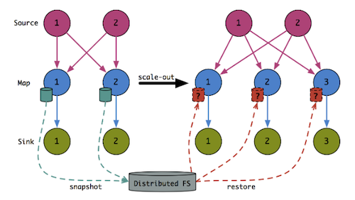
The key to support re-assigning state upon restoring from a checkpoint is to write the checkpoint with high granularity. More concretely, when a task saves a snapshot, for example some aggregation by key, it doesn’t do it as a monolith but rather as a collection at the key group level of granularity.
Thus when the system has to re-assign tasks it can look at the unified collection of aggregations across all tasks and redistribute it as it seems fit.
Implementation Details
State Storage
The snapshots must be persisted to some sort of database, which the paper calls state backend, and divides it into local state backend and external state backend.
In the local state case the data is stored locally, either in memory or out-of-core (can write to disk) using an embedded key-value database such as RocksDB. This enables data locality and doesn’t require coordination across multiple machines.
The external state can be further divided into non-MVCC and MVCC-enabled backends, where MVCC stands for Multi-Version Concurrency Control. For the non-MVCC case Flink uses a Two-Phase commit protocol with job manager as coordinator.
Individually, each task logs events to a local file (write-ahead log) and when a snapshot is requested, it sends a commit (“yes” vote) to the coordinator. Once all tasks submit their commits, the job manager commits the entire state atomically to the external DB.
MVCC-enabled allows commiting to different versions, so Flink maps epoch to these versions. This way task-level can commit snapshots without any explicit coordination. When all tasks have comitted, the external DB will update its current version.
Local vs external. While local state backends are simpler to write, they can be more difficult to read from during rollback, since the system needs to fetch the snapshot distributed accross all the machines. The paper suggests external backends is preferred when the state is large.
Asynchronous and Incremental Snapshots
The paper doesn’t provide much detail on this, but [6] does, so we use it to complement the discussion. Let’s focus on the out-of-core, local state backend case, in particular using RocksDB.
RocksDB is a key-value store which keeps a hash table in memory (called memtable). When the memtable gets too big, it is persisted to disk and no further state updates in done there and is now known as sstable.
Asynchronously, RocksDB merges two or more sstables into one to reduce the number of sstables in a process known as compaction. If the same key appears in multiple sstables, the one from the most recent sstable takes precedence. RocksDB thus implement a data structure called Log Structured Merge Trees or LSM, which we’ve discussed in the past [7].
Once the task running an instance of RocksDB receives a snapshot request, it first tells RocksDB to flush its memtable to disk and this is the only part done synchronously. Then it writes all the sstables since the last snapshot to a distributed file storage. By doing this, Flink is only storing the delta of sstables (i.e. incremental snapshotting). When it comes time to restore the state however, it needs to go over multiple snapshots to combine the data from all sstables.
One risk is that RocksDB will merge a sstable with another that has already been written to the distributed file storage (or snashotted), which would break the invariants regarding the incremental snapshots. To prevent this, Flink tells RocksDB to not merge sstables that haven’t been snapshotted yet.
Queryable State
Flink exposes a read-only view of its internal state to the application. One use case is to reduce latency in obtaining results, since by querying local state directly it can query fresh partial results. Flushing partial results frequently to the sinks would be prohibitive.
Each host running a task has a server that is capable of receiving requests from the application. The request includes the key to be looked up and the server returns the corresponding value. To reach the task containing the right set of keys, the request is first sent to the job manager which has the metadata to do the proper routing.
Exactly-Once Output
Because of recomputation, Flink might end up sending duplicated data to its sinks. To achieve exactly-once semantics it needs to do some extra work depending on the semantics provided by the sinks.
Idempotent sinks. can handle duplicated data, so no extra work is needed on Flink’s side. One example of a idempotent sink is a key-value store in which writing the same key-value one or multiple times has effectivelly no difference.
Transactional sinks. In case the underlying sink isn’t idempotent, Flink has to perform some sort of transaction so that it doesn’t output values until a snapshot is taken.
Experiments
The authors describe a real-world use case King.com and experiment with a few parameters to understand how snapshotting affects the pipeline performance.
They show that the time to snapshot increases linearly with the state size, but this doesn’t affect pipeline performance since it’s done asynchronously.
The alignment time depends on the parallelism because the more tasks in need of alignment, the higher the expected amount of wait time.
Conclusion
State management is hard. State management in an application that needs to run continuously in a distributed manner is even harder.
Snapshots and rollbacks allow us to abstract some of this complexity by turning the continuous processing into a discrete one. We just need to function properly until the next snapshot is taken.
The paper is well written but the space limitation makes it infeasible to provide details which makes some topics harder to understand such as incremental snapshots and and rescaling, but luckily they’ve been discussed in more detail in blog posts [5. 6].
References
- [1] State Management In Apache Flink: Consistent Stateful Distributed Stream Processing - Carbone et al.
- [2] NP-Incompleteness: [Paper] FlumeJava
- [3] NP-Incompleteness: Notes on Zookeeper
- [4] NP-Incompleteness: [Book] Streaming Systems
- [5] A Deep Dive into Rescalable State in Apache Flink
- [6] Managing Large State in Apache Flink: An Intro to Incremental Checkpointing
- [7] NP-Incompleteness: Log Structured Merge Trees
