kuniga.me > NP-Incompleteness > Log Structured Merge Trees
Log Structured Merge Trees
20 Jul 2018
In this post we’ll discuss a data structure called Log Structured Merge Trees or LSM Trees for short. It provides a good alternative to structures like B+ Trees when the use case is more write-intensive.
According to [1], hardware advances are doing more for read performance than they are for writes. Thus it makes sense to select a write-optimised file structure.
B+ Trees and Append Logs
B+ Trees add structure to data in such a way that the read operation is efficient. It organizes the data in a tree structure and performs regular rebalancing to keep the tree height small so that we never need to look up too many entries to find a record.
If the B+ Tree is stored in disk, updating it requires performing random access which is expensive for a spinning disk. Random access is order of magnitudes slower than sequential access in disk. Adam Jacobs [3] describes an experiment where sequential access achieves a throughput of ~50M access/second while a random access only 300 (100,000x slower!). SSDs have a smaller gap ~40M access/second for sequential access and 2000 access/second for random access.
The other extreme alternative to avoid disk seeks when writing is just to append content sequentially. We can do this by appending rows to a log file. The problem of this is that the stored data has no structure so searching for a record would require scanning the entire dataset in the worst case!
The LSM Tree aims to combine the best of both worlds to achieve better write throughput without sacrificing too much of read performance. The overall idea is to write to a log file but as the file gets too large, restructure the data to optimize reads. We can see it as a lazy data structure data gets updated in batches.
First we’ll describe the original version of LSM Trees and then an improved version with better performance for real world applications and used by databases like LevelDB [4].
LSM Trees
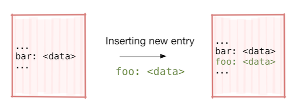
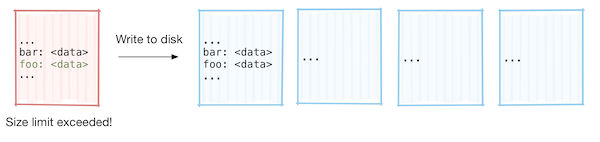
Let’s study LSM Trees applies to the implementation of a key-value database. Writes are initially done to an in-memory structure called memtable, where the keys are kept sorted (random access of RAM is not expensive). Once the table “fills up”, it’s persisted in disk as an immutable (read-only) file.
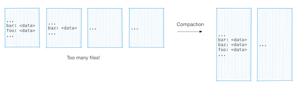
Searching for a key consists in scanning each file and within a file we can keep an index for the keys, so we can quickly find a record. Note that a key might appear in multiple files representing multiple updates to that key. We can scan the files by the most recent first because that would contain the last update to the key. The major cost of searching is due to the linear scanning of the files. As our database grows, the number of files will become too large to scan linearly.
To avoid that, once the number of files grow past a given number, we merge every pair of files into a new file using an external merge sort to keep the keys sorted. The linear factor of the search was cut in half, and while the file size doubled, the cost was sublinear, O(log n), so the search became twice as fast. This approach is known as tiered compaction [2].
The main disadvantage of this method is that once the files get past a certain size, the merge operation starts getting costly. Given m sorted files of size S, the merge operation would be O(m S log S). While this compaction will happen rather infrequently (roughly when the database doubles in size), it will take a really long time for that one time it happens.
This resembles the discussion of amortized analysis for data structures [5]. We saw that while amortized complexity may yield efficient average performance of a data structure, there are situations where we cannot afford the worst case scenario, even if it happens very rarely.
LSM with Level Compaction
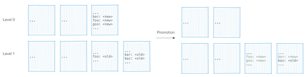
An alternative approach to work around expensive worst case scenarios is to keep the file sizes small (under 2MB) and divide them into levels. Excluding the first level which is special, the set of keys each two files at a given level contain must be disjoint, that is, a given key cannot appear in more than one file at the same level. Each level can contain multiple files, but the total size of the files should be under a limit. Each level is k times larger than the previous one. In LevelDB [4], level L has a (10^L) MB size limit (that is, 10MB for level 1, 100MB for level 2, etc).
Promotion. Whenever a given level reaches its size limit, one of the files at that level is selected to be merged with the next level or promoted. To keep the property of disjoint keys satisfied, we first identify which files in the next level have duplicated keys with the file being merged and then merge all these files together. Instead of outputting a single combined file like in the tiered compaction, we output many files of size up to 2MB. During the merge, if we find collisions, the key from the lower level is more recent, so we can just discard the key from the high level.
Details
When merging, to detect which files contain a given key, we can use Bloom filters for each file. Recall that a bloom filter allows us to check whether a given key belongs to a set with low memory usage. If it says the key is not in the set, we know it’s correct, while if it says it is in the set, then there’s a chance it is wrong. So we can quickly check whether a given key belongs to a file with low memory footprint.
The first level is special because the keys don’t need to be disjoint, but when merging a file from this first level, we also include the files where that key is present. This way we guarantee that the most up-to-date key is at the lowest level it is found.
To select which file to be merged with the next level we use a round-robin approach. We keep track of which file was merged last and then pick the next one. This can be used to make sure that every file eventually gets promoted.
When outputting files from the merge operation, we might output files with less than 2MB in case we detect the current file would overlap with too many files (in LevelDB it’s 10) in the next level. This is to avoid having to merge too many files when this file gets promoted in the future.
Cost Analysis
Since the files sizes are bounded to 2MB, merging files is a relatively cheap operation. We saw above that we can limit the file to not contain too many duplicate keys with the files at the next level, so we’ll only have to merge around 11 files, for a total of 11MB of data, so we can easily do the merge sort in memory.
The promotion might also cascade through the next levels since once we promote a file from level t to t+1, it might overflow level t+1, which will require another promotion as well. This in fact will be common because merging only moves off 2MB worth of data to the next level, so it will require a promotion the next time it receives a new file from the level below (ignoring the fact that keys get overwritten during the merge). Fortunately the number of levels L grows O(log n) the size of the data. So for LevelDB, where the first level size limit is 100MB, even for a disk with 100TB capacity, we would still need only about 8 levels.
Reads
The fact that each key belongs to at most one file at each level allows us to keep an index (e.g. a hash table in disk) of keys to files for each level. (This of course excludes the first level, but it has a small number of files, so linear search is not expensive).
One interesting property is that each level acts as some sort of write-through cache. Whenever a key gets updated, it’s inserted at a file at lower levels. It will take many promotions for it to be placed at a higher level with other files. This means that searching for a key that has been recently updated will require scanning very few levels or smaller indexes since it will be found at lower levels.
