kuniga.me > NP-Incompleteness > [Book] Streaming Systems
[Book] Streaming Systems
26 Jul 2022
In this post we will review the book Streaming Systems by Tyler Akidau, Slava Chernyak and Reuven Lax [1]. The book focuses on distributed streaming processing systems, reflecting the authors’ experience of building DataFlow at Google. Akidau is also one of the founders of Apache Beam.
We’ll go over some detail on each chapter. The notes might be missing context because I took them while I had the book in front of me, but I tried to fill some of it in as I noticed them. If you’re just interested in a summary, jump to the Conclusion.
Organization of the book
The book is divided in 2 parts for a total of 10 chapters. In Part I, the book covers the Beam model, which can be thought of a spec for how to implement stream processing systems and specifies high-level concepts such as watermark, windowing and exactly-once semantics. In Part II the authors provide the streams and tables view, which brings the concepts of batch and streaming closer together.
Most of the book is written by Akidau, with specific chapters written by Chernyak (Chapter 3) and Lax (Chapter 5).
Selected Notes
I’m going to over each chapter providing a brief summary interspersed with my random notes.
Chapter 1 - Streaming 101
In this chapter the author provides motivations for stream processing, introduces terminology and does some initial comparison with batch systems. This chapter is freely available online.
Cardinality: Bounded or Unbounded data. Bounded data have a determined beginning and end (i.e. boundary). Constitution: Table or Stream. Tables are a snapshot of the data at a specific point in time. Streams are element-by-element view of the data over time. Chapter 6 dives deeper into these. Constitution and cardinality are independent concepts, so we can have bounded stream and unbounded tables, but stream processing is mostly associated with unbounded streams. An event in a stream is the analogous to a row in a table.
Event vs. Processing Time. Event time is the timestamp corresponding to when the event was created (e.g. logged), while processing time is the timestamp when the event was processed by the system. Out-of-order data: one challenge with streaming is that events can come out-of-order (with respect to event time).
Completeness: with unbounded data, events can be arbitrarily late (e.g. event logged locally, offline, will only be processed when user goes back online). This makes theoretically impossible to know when we are done processing data.
Chapter 2 - The What, Where, When and How of Data Processing
This chapter introduces specific terminology and features from the Beam model including transformations, windows, triggers and accumulation. The Beam model concept is discussed in Chapter 10. This chapter is freely available online.
Transformations can be element-wise like a mapper, or change the data cardinality via aggregations such as group-by or widowing.
Watermark is a timestamp aiming to provide a boundary to unbounded data. It can be read as “I’ve already processed all events with timestamp less than the watermark”. This is important when events can be arbitrarily late because it provides a different criteria for moving on instead of waiting for all events to arrive. More details are covered in Chapter 3. Figure 1 shows the watermark lines as dashed/dotted line.
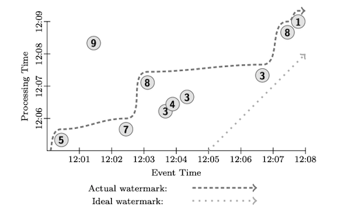
Triggers determine when to provide partial results when doing aggregations. For example, if we’re counting how many events match a given condition, we can setup a trigger that fires every 5 minutes, sending the current count downstream. Triggers can also be configured to fire when watermarks are updated.
Late data. Because we can move on without waiting for all data to arrive, it’s possible that some data arrives late. A late data is any event with timestamp less than the watermark.
Accumulation determines how to proceed with partial updates. Suppose we provide partial sums every 5 minutes. What should we do, while doing some aggregation, when the trigger fires a second time. There are a few options:
- Send the current partial sum
- Send a retraction of the previous partial sum and then a new one
- Send the delta
The choice of accumulation depends on the downstream consumer. If it’s writing to a key-value store, sending the current partial sum works well, but if it’s doing further aggregation it needs the retraction or the delta.
I found the “What, Where, When and How” view/analogy very confusing. Perhaps I didn’t internalize the right mental model, but I found it unnecessary.
Chapter 3 - Watermarks
This chapter dives deeper into watermarks.
Perfect watermark is one in which we have a guarantee that no event will be processed late. More precisely, let $t_{wm}$ be the current watermark. Perfect watermark says that for every event $e$ processed in the future, their timestamp $t_{e}$ will be greater than $t_{wm}$.
Perfect watermarks are impossible to implement in the general case because we cannot tell whether some event is stuck on a offline phone for example. Even if we could, waiting for a extremely late event could hold up the pipeline in case the trigger is configured to only fire when a watermark updates.
Heuristic watermarks allows trading off completeness (allowing some events to arrive late) for latency (reducing time waiting for laggards).
In multi-stage pipelines we need to keep track of watermarks at each stage because events can be processed in different orders (e.g. parallel mapper) or can be delayed due to system issues (crash, overload). In addition, some operations such as windowing naturally add a watermark delay. So for example if stage 1 performs a tumbling window of size 5 minutes, the next stage’s watermark is expected to be 5 minutes behind.
It’s possible to keep watermarks for processing time in addition to event time ones. This can be useful to detect if any stage is holding up the pipeline.
Chapter 4 - Advanced Time Windowing
This chapter dives deeper into windows.
Every aggregation in streaming processing is associated with a time window. For example, it doesn’t make sense to count the number of events in an unbounded stream without specifying a time range (i.e window).
Windows can be based on processing time, such as those associated with time-based triggers (e.g. fire every 5 minutes). They can also be based on event time, by leveraging watermarks. One example of event-time windowing is the tumbling window. Figure 2 shows an example.
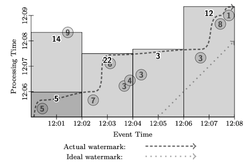
The tumbling window partitions the event time axis into fixed intervals. Events with timestamps inside the interval are considered part of the window. It’s possible to have multiple parallel windows, for example when we perform an aggregation following a group by key. In this case the tumbling windows can be aligned across all keys or they can be shifted to avoid burst updates when triggers fire.
Another type of window is data-dependent ones, for example session windows. Session windows are used to model user sessions. Events with the same key (e.g. user id) that happen within a duration from each other (say 5 minutes) are to be grouped in the same window.
Since the window boundaries are not known in advance, they must be merged on the fly. When windows are merged we likely need to perform retractions. Suppose we have a trigger that fires on every event processed. Suppose we currently have 2 session windows with range [10:00 - 10:05] and [10:10 - 10:30] and that the threshold duration for merging is 5 minutes.
Now a new event comes with event time 10:06. It will cause the windows to be merged into one with range [10:00 - 10:30]. However, the previous two windows had triggered outputs before so they need to retract those.
Chapter 5 - Exactly-Once And Side Effects
Exactly-once semantics is a guarantee that the consumer of the stream will see each event exactly once. This is in contrast with at-least-once semantics where each event is guaranteed to be included in the output but they could be included twice. And at-most-once where each event is guaranteed to not be duplicated but they can be dropped.
Exactly-once semantics is non-trivial to achieve in fault-tolerant systems because it has to retry computation while guaranteeing events don’t get processed twice.
Even if the system provides exactly-once guarantee, it doesn’t guarantee that the user function will be called exactly once (the guarantee is over the output), so if it’s non-deterministic or has side-effect, it can cause problems.
To achieve exactly-once guarantee the input of the system also needs to provide some guarantees. Either it has to have exactly-once guarantees itself or it must be able to identify events with a unique ID, so if the system can use it to detect duplicates itself.
Chapter 6 - Streams and Tables
In this chapter Akidau provides the theory of streams and tables. The idea is that both batch and stream processing use both streams and tables internally but in different ways.
I really like the physics analogy of table being data at rest, while stream is data in motion. Some transforms cause data in motion to come to a rest, for example aggregations, because they accumulate before proceeding to the next stage. Conversely, a trigger puts data at rest into motion, because it sends events downstream when the condition arrives.
I think an interesting analogy for aggregation of streams could be that of a dam. It accumulates water and lets some of it flow downstream. I don’t recall seeing this in any materials I read so far, though there’s the leaky bucket algorithm for rate limiting, which has the spirit of a dam, albeit at a smaller scale.
Chapter 7 - The Practicalities of Persistent State
This chapter discusses checkpoints, which provides a way to achieve at-least-once or exactly-once semantics. The idea is to write computed data to a persistent state periodically so it can be recovered in cases of failures.
Persistence is often applied when aggregations such as group by happens. This is because data needs to leave the machine it’s currently in to be sent to the next stage (i.e. shuffling, like in MapReduce).
Depending on what kind of aggregation we perform, we need to store more or less data. At one end of the spectrum is a simple list concatenation, which essentially involves storing every single event to a persistent state. On the other side is an aggregation into a scalar, much cheaper to store, but it restricts which aggregations can be used (must be associative and commutative).
Beam provides a very custom API that allows reading and writing to shared state inside user functions. Akidau provides a case study which to track conversion attribution, which involves traversing a tree.
Chapter 8 - Streaming SQL
In this chapter the author builds upon the unified view of streams and tables and proposes a unified SQL dialect that supports both batch and stream processing.
It introduces the concept of Time-Varying Relation (TVR) which is basically a series of snapshots of a table over time, each time it is modified. A table represents one of these snapshots at a given time, while a stream is the delta of changes, i.e. different views of the same thing.
With that model in mind, a hypothetical SQL dialect would allow users to specify which view to get via a modifier. For example, for a table view:
SELECT TABLE
  name,
  SUM(score) as total,
  MAX(time) as time
FROM user_scores
GROUP BY name;
Possible output:
| name  | total | time  |
| ----- | ----- | ----- |
| Julie | 8     | 12:03 |
| Frank | 3     | 12:03 |
For a stream view, we would have almost the same syntax but with different default semantics. One interesting bit is that because stream processing can do retractions (see Chapter 2 and Chapter 4), a system-level column exists indicating whether a row is a retraction:
SELECT STREAM
  name,
  SUM(score) as total,
  MAX(time) as time,
  Sys.Undo as undo
FROM user_scores
GROUP BY name;
Possible output:
| name  | total | time  | undo |
| ----- | ----- | ----- | ---- |
| Julie | 7     | 12:01 |      |
| Frank | 3     | 12:03 |      |
| Julie | 7     | 12:03 | true |
| Julie | 8     | 12:03 |      |
..... [12:01, 12:03] .........
The last line indicates the stream is not over, but that the rows shown is over a specific time interval.
Chapter 9 - Streaming Joins
This chapter build on the SQL syntax to introduce Streaming joins, that is, joining two streams based on a predicate. Akidau describes many variants of joins like FULL OUTER, INNER, LEFT, etc, and that all variants can be seen as a special case of FULL OUTER.
From the perspective of the stream-table theory, join is a grouping operation which turns streams into a table (puts data at rest).
A common pattern is to join on two keys being equal and to define a time range (window) for the joins to happen, but in theory stream joins can be “unwindowed”.
It has the same challenges as stream aggregations, namely dealing with out-of-order data. To work around that we also need to leverage watermarks and retractions.
Chapter 10 - The Evolution of Large-Scale Data Processing
This chapter reviews some distributed systems that inspired the current state-of-the-art for stream processing. It mentions Map-Reduce, Hadoop, FlumeJava, Storm, Spark Streaming, Millwheel and Kafka.
It culminates with Data Flow (at Google), Flink (open-source), and the Beam model (sort of a high-level spec which Data Flow and Flink try to adhere to).
Conclusion
I found the visualizations and diagrams one of the highlights of the book. There were a lot of aha moments when looking at the figures after trying to wrap my head around some concept. There are many reviews in Goodreads complaining the visualizations are subpar because they were made to be animated and don’t fit well in print. I personally didn’t find them an issue.
The stream and table theory and the surround analogies with concepts in physics was elucidating.
I liked the fact the authors were upfront about which person wrote each chapter. I recall having a bad experience reading Real World Haskell because the writing between chapters varied widely. Having known who wrote what would help to set expectations, perhaps even to decide whether to skip chapters.
As mentioned in my Chapter 2 notes, I found the “What, Where, When and How” view/analogy very confusing.
Related Posts
- [Book] Designing Data Intensive Applications - Martin Kleppmann’s book discusses practical distributed systems more broadly but it does have a section on stream processing. He also provides a view of stream and tables, including the calculus analogy: stream being the derivative of tables and tables the integral of streams.
References
- [1] Streaming Systems by Tyler Akidau, Slava Chernyak and Reuven Lax
- [2] The Dataflow Model: A Practical Approach to Balancing Correctness, Latency, and Cost in Massive-Scale, Unbounded, Out-of-Order Data Processing - by Akidau et al.
