kuniga.me > NP-Incompleteness > Huffman Coding
Huffman Coding
11 Jun 2020
David Albert Huffman was an American pioneer in computer science, known for his Huffman coding. He was also one of the pioneers in the field of mathematical origami [1].
Huffman, in a graduate course was given the choice of a term paper or a final exam. Students were as_ked to find the most efficient method of representing data using a binary code.
Huffman worked on the problem for months, but none that he could prove to be the most efficient. Just as he was about to give up and start studying for the finals, the solution came to him. “It was the most singular moment of my life”, Huffman says.
“Huffman code is one of the fundamental ideas that people in computer science and data communications are using all the time”, says Donald E. Knuth [2]. In this post we’ll study the Huffman coding algorithm and analyze it’s complexity and efficiency in terms of information theory.
Problem
Given a text T and a table of probabilities of occurrence of each symbol, find a lossless encoding that approximates the optimal theorical encoding (which we’ll define later).
Algorithm
The idea is to construct a binary tree known as Huffman tree from symbols frequencies. Each symbol from T is represented by a leaf and the path from the root will determine its encoding. More precisely, taking a ‘left’ corresponds to a 0 in the path, while taking a ‘right’ corresponds to 1.
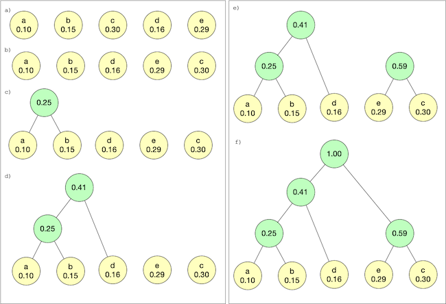
To construct the tree we first create nodes for each symbol, with a value equal to the symbol’s probability. Then we pick the two nodes with the smallest frequencies and connect them using a parent node, whose value will be the sum of its two child values. Repeat until there’s a single node, which will be the root.
Priority Queues. This can be implemented by using a priority queue ordered by the value. The smallest two values will be in front.
Two Queues. Wikipedia [1] and Knuth [3] also propose a solution using two queues, which I haven’t heard of before, but it’s pretty neat.
We have Q1 and Q2, Q1 starts with all nodes and Q2 is empty. When looking for the smallest value, we look at the front items of each queue and pick the smallest. Repeat to find the next smallest. Always insert the newly formed node at the end of Q2.
This idea coded in Python looks like:
def build_tree(frequency_map):
    frequency_map = sort_map_by_value(frequency_map)

    nodes = []
    for [symbol, f] in frequency_map.items():
        node = Node.symbol(f, symbol)
        nodes.append(node)

    q1 = Queue(nodes)
    q2 = Queue()

    def get_min(q1, q2):
        if less(q1.front(), q2.front()):
            return q1.pop()
        else:
            return q2.pop()

    while q1.len() + q2.len() >= 2:

        x = get_min(q1, q2)
        y = get_min(q1, q2)
        s = Node.combine(x, y)
        q2.push(s)


    return q2.front()
For the sake of code simplicity assume front() returns None if the queue is empty and the operator less() assumes None is infinite. Note we never have both operands equal to None since Q1.length + Q2.lengh >= 2. The complete implementation is on my github.
Let’s get some intuition on why using two queues is a correct implementation. We need to prove that each step x and y are the nodes with the smallest frequencies over all nodes.
Suppose that the queues store only the frequencies instead of the nodes. At a given iteration our queues are:
\[Q1 = [ai, a_{i+1}, …, a_n] \\ Q2 = [s_j, s_{j+1}, …, s_k]\]Our invariant is that:
- 1) both queues are sorted and
- 2) \(s_k\) was obtained by adding the smallest of \([a_{i-2}, a_{i-1}]\), \([a_{i-1}, s_{j-1}]\) or \([s_{j-1}, s_{j-2}]\).
Now let’s execute a step: we’ll either combine \((ai, a_{i+1})\), \((ai + s_j)\) or \((s_j, s_{j+1})\), the one that is the smallest of them (by our invariant we know that one of these have to be the smallest). We’ll call the result \(s_{k+1}\) and by construction our invariant (2) is kept.
Q1 is still sorted since we’re not adding elements to it. What remains is to show \(sks_{k+1} \ge s_ksk\). Let’s consider the 3 possibilities:
- \(s_{k+1} = [a_i, a_{i+1}]\): we know by invariant (2) \(s_k \le [a_{i-2}, a_{i-1}]\). Since \(a_i \ge a_{i-2}, a_{i+1} \ge a_{i-1}\) by invariant (1), \(a_i +a_{i+1} \ge a_{i-2} + a_{i-1}\), so \(s_{k+1} \ge s_k\)
- \(s_{k+1} = a_i + s_j\): we can use a similar argument since \(s_k \le [a_{i-1}, s_j-1]\) and \(a_i \ge a_{i-1}\) and \(s_j \ge s_j-1\).
- \(s_{k+1} = s_{j-1} + s_{j-2}\), we can use a similar argument.
If both invariants hold, we can see that \(s_k\) is the minimum sum of pairs of elements of either Q1 or Q2, proving the correctness of the approach.
Encoding
Before we encode the text, first we traverse the tree to build a mapping from each symbol to their corresponding path.
def build_lookup(tree):
    def traverse(node, path, lookup):
        if node.symbol:
            lookup[node.symbol] = path[::] # clone
        else:
            # To be efficient, update path in place...
            path.append(0)
            traverse(node.left, path, lookup)

            path[-1] = 1
            traverse(node.right, path, lookup)

            # ...but restore it once done
            path.pop()

    lookup = {}
    traverse(tree, bitarray(), lookup)
    return lookup
Note that we used a bit-array to save space (using ‘0’/’1’ characters would defeat the purpuse since it would use 8 bits where we only need 1).
Then we can simple iterate over all symbols in the text:
def encode(text, tree):
    lookup = build_lookup(tree)
    encoded = bitarray()
    for c in text:
        code = lookup[c]
        encoded.extend(code)
    return encoded
Decoding
In a Huffman tree all the nodes that encode a symbol are leaves. This makes the Huffman encoding prefix free. For example, if a given symbol S is encoded by path P, there’s no prefix of path P that encodes another symbol S’ because this would imply symbol S’ is encoded by a non-leaf node.
This property is important because it makes decoding unambiguous. If we receive a Huffman-encoded message M = [b1,b2,...,bn], and we find out a symbol encoded by the path: Pk = [b1, b2, …, bk], we know no other symbol is encoded by a prefix of Pk, and we know Pk is not a prefix of some larger prefix. This leads to a very simple way to decode a Huffman tree.
We use the encoded binary data as directions until we find a symbol, in which case we restart at the root.
def decode(encoded, tree):
    node = tree
    text = ''
    for bit in encoded:
        if bit is False:
            node = node.left
        else:
            node = node.right

        if node.symbol is not None:
            text += node.symbol
            node = tree

    return text
In practice, if we are sending a encoded message over to a receiver, they will need to have access to the tree, either by reconstructing it from the symbols and their probabilities, or by sending the tree itself as part of the message, in case the eencoded message is really big.
Theory
Before we start studying the proofs from a theoretical point of view, let’s establish some conventions. Whenever we refer to \(\log(x)\) it will represent the logarithm of \(x\) in base 2.
Information Theory and Entropy
Information Theory was pioneered by Claude Shannon as one outcome of trying to optimize the transmission of information. One of the most important concepts in information theory is the concept of entropy [4].
Entropy can be regarded as the amount of information necessary to represent some source of information. In the context of communication, we can define the entropy of a source of information (a sender). In an idealized model, this source sends some amount of information per second over an infinite amount of time (i.e. continuous stream). We also assume the properties of the data (e.g. the relative frequency of characters) doesn’t change over time. Such source is called ergodic.
It helps to think of entropy in terms of a channel capacity between a sender and a receiver. We want to know what is the minimum bandwidth (in bits/s) a channel would need to have to be able to transmit the data from the client to the server.
Let’s workout some examples to make the notion more intuitive. Suppose our source emits one binary digit per second. What would be the capacity of our channel? We know from data types such as byte, int32, int64 that the distinct numbers we can represent is \(2^{bits}\), so for example a byte (8 bits) can represent \(2^{8} = 256\) values. Conversely the number of bits to represent k values is given by \(\log(k)\).
Thus, for a source emitting two values per second (0 or 1) we need exactly \(\log(2)\) = 1 bit/second. Now imagine that the source only emits 1. How many bits do we need? Since it’s one value, we need \(\log(1)\) = 0 bits/second. That’s right, we don’t need to send any information at all! The receiver will know the source has this property and doesn’t need to receive information to know what is coming!
More generally, if bit 0 has relative frequency \(p_0\) and one has relative frequency \(p_1\), the entropy of the source his given by \(E = -p_0\log(p_0) -p_1\log(p_1)\). So for a random case \(p_0=\frac{1}{2}\) and \(p_1=\frac{1}{2}\) we have \(E = -\frac{1}{2} \log(\frac{1}{2}) - \frac{1}{2} \log(\frac{1}{2}) = 1\). when all digits are 1, \(p_0 = 0\) and \(p_1 = 1\). While \(\log(0)\) is undefined, \(xlog(x)\) converges to 0 as \(x\) goes to 0, so we get \(E=0\).
Let’s consider another case where \(p_0 = \frac{3}{4}\) and \(p_1 = \frac{1}{4}\). Then \(E=0.81\), less than 1 bit/s. For a source with \(n\) symbols, the entropy can be generalized to:
\[H = \sum_{i=1}^{n} p_i \log(p_i) \quad (1)\]Huffman Tree is optimal
We’ll now show that Huffman trees minimize the following function:
\[\sum_{i=1}^{n} p_i l_i \quad (2)\]where \(l_i\) is the length of the path from the root to node \(i\).
We’ll describe the proof provided by Knuth in [3], based on induction on the number of symbols \(n\), that is, suppose we know how to construct a tree with \(k < n\) weights.
Let be a minimal tree of size \(n\) and \(V\) the internal node with largest height. Let \(w_i\) and \(w_j\) be the children of such node. We can swap the children of \(V\) with \(w_1\) and \(w_2\) without increasing the objective function. So we can asume an optimal tree exist where \(V\) has \(w_1\) ans \(w_2\) as children.
Combine \(V\), \(w_1\) and \(w_2\) into one note with weight \(w_1+w_2\). Now, construct an optimal tree for weights \(w_1+w_2, w_3, …, w_n\), which we know how to do since it has \(n-1\) weights. Such tree has a leaf node with weight \(w_1+w_2\). We can “expand” that node into one with children \(w_1\) and \(w_2\). The cost of this function is \(U = T + w_1 + w_2\).
If \(T\) is optimal, then \(U\) is optimal. If not, there’s \(U^* < U\), by our first argument we can find another tree with cost \(U^*\) having \(w_1\) and \(w_2\) as children, by “shrinking” then into \(w_1+w_2, w_3, ... , wn\), we could find a tree with cost \(< U - w_1 - w_2 = T\), contradicting the fact \(T\) is optimal. QED.
Now, does the Huffman Tree minimize the entropy as defined by information theory? As we recall, the entropy is defined as (1)
\[H = - \sum_{i=1}^{n} p_i \log(p_i)\]not quite the same as (2)
\[\sum_{i=1}^{n} p_i l_i\]In practice there are examples where the entropy (1) is less than that of (2) (See Experiments).
Shannon Encoding. Shannon proposed an encoding where the length of each code has length \(\lceil-\log (p_i)\rceil\) (this is also mistakenly known as the Shanno-Fano encoding [5]). We’ll not go over the specifics here but it can be shown to be a prefix-free binary encoding. The entropy of such encoding is given by (2). In this case, \(l_i = \lceil-\log (p_i)\rceil \le -\log (p_i) + 1\). Using this in (2):
\[\sum_{i=1}^{n} p_i l_i \le \sum_{i=1}^{n} p_i (-\log (p_i) + 1) = - \sum_{i=1}^{n} p_i \log (p_i) + \sum_{i=1}^{n} p_i = H + 1\]Every binary encoding that is prefix-free can be represented by a binary tree where the symbols are on the leaves. This is just the same sort of tree that Huffman is optimal for, so we can claim that the Huffman tree is no worse than “Shannon’s tree” in terms of minimizing (1). Hence, \(H + 1\) is also a upper bound for the entropy of a Huffman encoding.
We have shown that while Huffman encoding doesn’t always achieve the lowest theoretical minimum for entropy, it’s within 1 bit from it. By grouping blocks of symbols and encoding them together instead of symbol by symbol it’s possible to reduce the difference further.
Experiments
We tried out the Huffman encoding with a real-world example. Jane Auten’s Pride and Prejudice. This is a classical work available for free. It contains about 774K characters (including punctuation and spaces), and 124k words.
We used the character frequency of the text to build the Huffman tree. We then calculate the entropy and compare the size of the compressed and uncompressed texts.
Entropy:
- Theoretical Minimum: 4.29
- Huffman: 4.32
We can see that it’s consistent within the expectations: the Huffman entropy is very close (0.7%) but not as optimal as the theoretical minimum, but it’s within a bit of 4.29.
If we measure the size of the text in bytes vs the compressed bitarray:
- Raw text: 774 Kbytes
- Huffman encoded text: 417 Kbytes
The compression rate is 1.85.
As we mentioned before, encoding blocks of characters yields more efficient encodings (at the cost of bigger Huffman trees and lookup tables). We can use words as symbols instead of characters. To simplify things we remove punctuations and multiple spaces “the dog ‘barked’.” becomes “the dog barked”.
Entropy per character (assuming an average of 4.5 characters):
- Theoretical Minimum: 2.120
- Huffman: 2.126
The Huffman entropy is now within 0.28% of the optimal.
For the raw text, the size will be the sum of length of all words plus one extra byte per word since we’d need to distinguish between them (e.g. by adding a space).
- Raw text: 681 Kbytes
- Huffman encoded text: 148 Kbytes
The compression rate is 4.6.
Conclusion
I’ve learned about Huffman coding a while back during a data structures class, but I don’t recall really understanding the efficiency in term of entropy. I was motivated to revisit this topic after reading “Introduction to Information Theory” by John Pierce. It’s an accessible book that discusses Information Theory at large.
Interesting fact: I found many bugs in my initial implementation by checking two invariants: one is that encoding + decoding a text should yield the original text, that is: T = decode(encode(T)). The other is that the entropy of the Huffman encoding should be within 1 bit of the optimal entropy.
