kuniga.me > NP-Incompleteness > Bloom Filters
Bloom Filters
29 Jan 2015
Burton Howard Bloom is a MIT alumni, who, mwhile employed by the Computer Usage Company, developed and published a data structure that later became famous as “Bloom Filter” [1].
In this post we’ll talk about Bloom Filters. We’ll give a description of the data structure and its operations. We’ll then study the theory that explains the performance of this data structure. Next, we’ll describe an implementation in Python, run some experiments and finally discuss applications.
Introduction
Bloom filter is a probabilist data structure that enables inserting elements in a set and test whether an element belongs this set, sacrificing accuracy for lower memory usage.
More precisely, it can say an element is in the set when in fact it’s not (false positive), but if it says it’s not in the set, then it’s true. Also, the original variant doesn’t allow removal of elements [2].

In its original form, it doesn’t allow removing elements.
Algorithm
The bloom filter structure consists of a bit array of size \(m\). We then define k independent hash functions, which can distribute a given value into any of the \(m\) positions uniformly.
Inserting an element consists in applying the \(k\) hash functions to the element and set the bit in the \(k\) positions returned by these functions to 1.
Querying for an element consists in applying the same \(k\) hash functions and testing whether all the bits in the k positions returned by these functions is set to 1.
If the test returns positive, there’s a chance the element is there, but it could be a false positive, since the bits could have been set by the insertion of other elements. On the other hand, if it returns negative, we’re sure the element is there, because we never unset a bit. Also, as the number of elements in the set grow, the probability of false positives increases.
Time complexity. Both insertion and querying for an element are constant-time operations, since they are proportional to \(k\), assuming random access memory and \(O(1)\) hash functions.
Probability of false positives. The probability \(p\) that the algorithm will return true when the element is not there (false positive), can be described in terms of \(m\), \(k\), \(n\), through the following equation:
\[(1) \quad p = \paren{1 -e^{-(kn/m)}}^k\]In Appendix A, we provide an approximated derivation of this result.
Optimal number of hash functions. For given values \(n\) and \(m\), we have a choice of how many hash functions to use, \(k\). Intuitively, if we use too few hash functions, we may increase the chances of collision when querying for an element, whereas if we use too many, the array will be filled up earlier and thus the collisions will also increase.
It’s possible to prove (a proof is sketched in appendix B), that for fixed \(m\), \(n\), the value of \(k\) that minimizes \(p\) is given by:
\[k = \ln(2)m/n\]Replacing in $(1)$ gives us:
\[p = \paren{1 -e^{-(\ln(2))}}^k = \paren{\frac{1}{2}}^{\ln(2)m/n} = 2^{-\ln(2)m/n}\]With $2^{-\ln(2)} = 0.6185$, the optimal probability of false postives is thus:
\[p = 0.6186^{m/n}\]Python Implementation
In this experiment, we use the bitarray python module. It’s a C implementation that represents a bit array efficiently. It has conveniently overloaded operators so most of the time it’s like working with arrays.
We can define a sufficiently large value of our bit array length, \(m\), for example:
from bitarray import bitarray
m = 1 << 20
bit = bitarray(m)

# bitarray doesn't guarantee the bits are all set to 0
# upon initialization
bit.setall(False)
The murmur algorithm
We need to pick a hash function to use with our Bloom filter. References such as [3] suggest using an algorithm called Murmur. This stack exchange thread has a nice survey about different hash functions.
Murmur is a hash algorithm developed by Austin Appleby. Even though it’s not suitable for cryptographic applications, in practice it is very fast and tends to distributed real world instances well.
According to the author, the name comes from an early implementation detail, which used multiply-rotate-multiply-rotate operations to mix the internal state of the hash (hence MuR-MuR).
From the source code, this algorithm seems to shuffle the bits from the input key by using multiplication, shifting and xor operations.
The author mentions using simulated annealing to find some of the constants of the final mix of algorithm. This final part is used to cause the avalanche effect, in which very similar inputs are hashed to very different values.
There’s is a Python library called mmh3 that has an interface for several hash functions (implemented in C++).
To install it, we can use pip:
pip mmh3To use it within a Python script:
from mmh3 import hash128
hash_value = hash128(input)
Families of hash functions
In Jonathan Ellis’s post, he mentions a strategy for generating a family of hash functions. He cites a paper from Kirsch and Mitzenmacher [4] which shows we can generate a set of \(k\) hash functions from 2 independent hash functions in the following way:
\[h_k(x) = h_A(x) + i \cdot h_B(x), \, i = 0, \cdots, k-1\]In practice, since murmur3_x64_128() generates 128-bit hashes, we can use the first 64-bits as the first hash function, and the last 64-bits as the second.
from mmh3 import hash128

h128 = hash128(input)
h64l = h128 & ((1 << 64) - 1)
h64u = h128 >> 64

hashes = map(
  lambda i: (h64l + i*h64u) % k,
  range(k)
)
All the code is available on github.
Experiments
Before running experiments with our Bloom filter implementation, let’s try to visualize the distribution of the Murmur hash functions. For this first experiment, we compute the hash function of keys ranging form 1 to 10k and module it 10k, so they’re all in the same range of values. Then we plot the keys vs. their hashes in a scatter plot, by exporting this data as a CSV file and rendering in R (using ggplot2):
ggplot(data, aes(x=i, y=h_i)) + geom_point(size=1.5)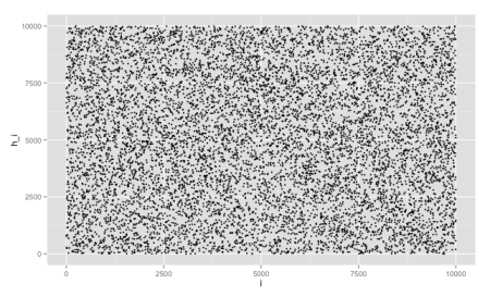
From the chart, we can see it apparently distributes the keys uniformly, without any obvious pattern. This is not sufficient to prove it’s a good hash function, but it’s a necessary property.
To test the family of hashes, we can add a new column, which has i for the i-th hash function. Then, in ggplot, we render each class with a different color with the following command:
ggplot(data, aes(x=i, y=h_i, color=class))
  + geom_point(size=1.5) + facet_grid(class ~ .)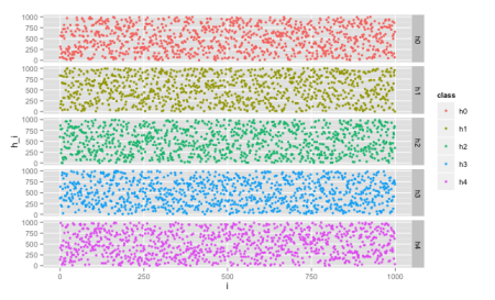
We can now compare the distributions between each of the hashes by plotting scatter plots for each pair i, j. Now we use another ggplot2 command to generate a 5x5 grid of charts:
ggplot(data, aes(x=i, y=h_i, color=class))
  + geom_point(size=1.5) + facet_wrap(~class, ncol=5)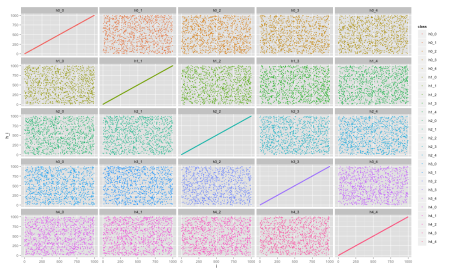
We can see each chart has a uniform pattern, which is a good sign if we’re looking for independent hash functions. For comparison, let’s plot the same chart for a set of hash functions derived only from a single hash function, for example
\[h_i(x) = i \cdot h_A(x), i = 1, \cdots, k\]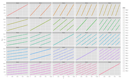
Now, let’s analyze the false positive rate. We can do that by counting the number of false positives FP and the true negatives TN and evaluating:
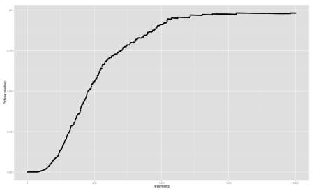
\[\dfrac{FP}{FP + TN}\]We fix \(m\) and \(k\) and shuffle an array from 0 to n-1 to simulate a sampling without replacement. After each inserted element of this array, we go over all non-inserted elements \((FP + TN)\) and count how many of those our Bloom filter thinks they are in the set \(FP\). We then plot a line chart with the number of elements inserted vs. the false positive rate, using qplot() R function:
qplot(
  data$n,
  data$prob,
  ylab='Pr(false positive)',
  xlab='N elements'
)
Let’s plot the effect of increasing the size of the bit array, using the optimal k and increasing the number of elements. In this particular experiment, we use n=250 and try different values of m: 100, 250, 500, 1000
qplot(
  data$n,
  data$prob,
  ylab='Pr(false positive)',
  xlab='N elements',
  size=I(1),
  color=data$m
) + scale_colour_manual(
  values=c("red", "blue", "green", "black"),
  name="m values"
)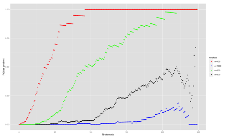
One strange behaviour seems to happen towards the right end of the chart for some curves – the false probability ratio seems to drop. I’ve double checked the code and it looks sane. One possible explanation is that we are calculating the probability over the non-inserted elements and as it approaches the end, the sample size is smaller, so the noise is more significant. Other than that, the probability of false positives tend to increase as we add more and more elements.
Now, let’s analyze the effect of the number of hash functions used. We fix it in n=250, m=1000 and try out different values of k=1, 5, 10, 50.
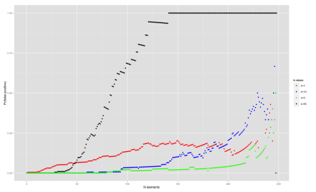
We can see that using many hash functions can be bad because it fills up the array too fast (k=50). In general k=5 and k=10 perform best for most part of the spectrum.
Applications
Bloom filters are suitable where false positives are tolerable. For example, it can be used as a first step to avoid lookup to a cache. Periodically a cache server could send a Bloom filter to a local machine, corresponding to items it has cached. If the Bloom filter says an element is on cache, it might not be true, but if it says the item is not there, the local client can avoid a request to the cache and talk directly to the underlying storage.
Bloom filters use little memory, so they are suitable for network transmission.
Broder and Mitzenmacher discuss a lot more examples [5], especially network applications.
Conclusion
In this post we learned about Bloom filters. The idea itself is quite simple, by studying the theory we are able to review some probability and calculus concepts.
The implementation made us aware of details which are usually not discussed in theoretical texts, for example, which hash functions to use and how to generate a family of hash functions.
We used two Python libraries, pyhash and bitarray and learned a little bit about the Python packaging system, PyPI. We got some experience with the ggplot2 R library, which I plan to post about later.
What we didn’t cover was variants of Bloom filters, like the count version, which allows deletion. Chazelle et al., introduced the Bloomier Filters, which is a generalization of Bloom filters [6].
References
- [1] Quora - Where can one find a photo and biographical details for Burton Howard Bloom, inventor of the Bloom filter?
- [2] Wikipedia - Bloom Filter
- [3] Spyved - All you ever wanted to know about writing bloom filters
- [4] Less hashing, same performance: Building a better Bloom filter - A Kirsch, M. Mitzenmacher.
- [5] Network Applications of Bloom Filters - A. Broder, M. Mitzenmacher
- [6] Bloomier Filters - B. Chazelle et al.
- [7] Probability and Computing: Randomized Algorithms and Probabilistic Analysis - M. Mitzenmacher, E. Upfal
Appendix A: Probability of false positives
Let’s consider an array of m bits and the insertion operation. The probability of a given bit to be set by one of the hash functions is \(1/m\). Conversely, the probability of a bit not being set is \(1 - 1/m\). By the hypothesis of independent hash functions, the probability of a bit not being set by any of the \(k\) hash functions is
\[\left(1 - \frac{1}{m}\right)^k\]Inserting \(n\) elements is equivalent to running the \(k\) functions \(n\) times, so after inserting \(n\) elements, the probability that a given bit is set to 0 is
\[\left(1 - \frac{1}{m}\right)^{kn}\]or the probability it’s set to one as
\[1 - \left(1 - \frac{1}{m}\right)^{kn}\]Now, the probability of a false positive \(p\), is the probability \(k\) positions being set for a element that was never inserted.
\[(2) \quad p = \left(1 - \left(1 - \frac{1}{m}\right)^{kn}\right)^k\]According to [2] though, this derivation is not accurate, since assumes that the probability of each bit being set is independent from each other. The Wikipedia article sketches a more precise proof from Mitzenmacher and Upfal [7] which arrives at the same result.
To simplify the equation, we’ll use the following identity:
\[\lim_{x\to\infty} \left( 1 - 1/x \right)^x = 1/e\]So, for large values of $m$, we can assume that
\[(1 - 1/m)^{kn} = ((1 - 1/m)^m)^{(kn)/m} \approx (1/e)^{(kn/m)} = e^{-(kn/m)}\]Replacing it in $(2)$ we have:
\[p = \paren{1 - e^{-(kn/m)}}^k\]Appendix B: Optimal number of hash functions
If we make \(p\) a function of \(k\), it’s possible to prove it has a global minimum for positive \(k\)’s so we can use the derivative to find the value of \(k\) that minimizes the false positive probability.
To find the derivative, we can use the generalized power rule to get
\[\ln(1 - e^{-ck}) + \frac{k}{(1 - e^{-ck})} c e^{-ck}\]where \(c=n/m\) is a constant. If we make \(y = e^{-ck}\) (and use \(k = \ln(y)/-c\))
\[\ln(1 - y) - \frac{\ln(y)}{(1 - y)} y\]By making it equals to 0, we get the equation:
\[\ln(1 - y) (1-y) = \ln(y) y\]To solve this for \(y\), let \(x = 1 - y\),
\[\ln(x) x = \ln(y) y\]Since \(\ln(n)\) and \(n\) are both monotonic functions, so is \(\ln(n)n\). Then if () holds, we can conclude that \(x = y\), because otherwise, if \(x > y\), \(\ln(x) x > \ln(y) y\) and if \(x < y\), \(\ln(x) x < \ln(y) y\).
Replacing \(x\) back, we find out that \(y = 1/2\) and finally \(k = ln(2)m/n\).
