kuniga.me > NP-Incompleteness > Linear Predictive Coding in Python

Linear Predictive Coding in Python

13 May 2021

Linear Predictive Coding (LPC) is a method for estimating the coefficients of a Source-Filter model (post) from a given data.

The input consists of a time-series representing amplitudes of speech collected at fixed intervals over a period of time.

The output is a matrix of coefficients corresponding to the source and filter model and is much more compact, so this method can be used for compressing audio.

In this post we’ll study the encoding of a audio signal using LPC, which can achieve 15x compression. We’ll then decode it into a very noisy but intelligible speech.

This study is largely based on Kim’s excellent article, which also provides the code in Matlab.

The contribution of this post will be:

• Use Python instead of Matlab. Reason: Matlab is not free - I know of Octave and used it for this post to understand differences between Python and Matlab APIs, but I also wanted to learn about the Python libraries.
• Start from the code and provide the theory behind it. Reason: As someone not familiar with signal processing, I found it non-trivial to go from the theory to the code, so I’m hoping this approach can be useful.

Audio Processing

In this section we’ll read the input signal from a file and pre-process it to a suitable format.

Digital Audio

Audio is a physical, analog phenomena which must be represented digitally (discrete) in a computer.

To convert an analog signal to a digital one, we need to obtain discrete samples. We usually work with sample rate, the number of samples per second which is given in Hertz. If we have too few samples, we’ll not correctly represent the signal. If we have too many, we’ll end up using more storage than needed. As an example, the sample rate of CD-quality audio is 44.1 kHz, that is, 44,100 samples per second.

Audio Format vs File Format

These terminologies can be confusing since they’re often used interchangeably. File formats are the user facing ones, for example WAV (Waveform Audio File Format) and MP3 (MPEG-2 Audio Layer III). They have an associated file extension, for example .wav and .mp3.

The audio format is associated to how audio data is represented (encoded) in a file. We have PCM (Pulse-code modulation) which is how WAV encodes its data, and MP3 which is both an audio and file format.

Some file formats can work with multiple audio formats, for example the MP4 file format, which supports audio formats like ALS, MP3 and many others.

To make it more clear, when we’re referring to file formats we’ll use the extension (.mp3).

Reading .wav file

We’re ready for our very first task: read a .wav file to memory. We can use the scipy library:

import scipy.io.wavfile

...

[sample_rate, pcm_data] = scipy.io.wavfile.read('lpc/audio/speech.wav')

The read() function returns the sample rate in which the file is encoded and the data itself. For this post we’ll assume our audio has a single channel so that pcm_data is simply an array containing the amplitude of each samples.

Numpy Arrays

We’ll be using numpy a lot for matrix operations, so it’s better to work with numpy data structures all times, hence the np.array() conversion.

import numpy as np
amplitudes = np.array(amplitudes)

Dimensions. One of the critical parts of working with numpy arrays is understanding its dimensions. Numpy arrays are multi-dimensional, which can be inspected via the shape attribute. Some examples:

# 10 x 10 matrix
m = np.empty(shape=(10, 20))
print(m.shape) # (10, 20)
# vector of size 10
v = np.empty(shape=10)
print(v.shape) # (10, )
# 10 x 1 matrix
m = np.empty(shape=(10, 1))
print(m.shape) # (10, 1)

Note the difference between the 1 dimensional vector (10, ) and the 2 dimensional matrix with one column (10, 1).

Let’s inspect our amplitudes:

print(amplitudes.shape) # (530576, )

which shows it’s a vector with ~500k elements.

Normalizing Amplitude

We want to work with amplitudes within [-1.0, 1.0] so it’s easier to visualize and compare signals.

amplitudes = 0.9*amplitudes/max(abs(amplitudes))

Numpy arrays work with list functions like max() and abs(). It also differs from regular list in operators like * and /, where it performs the operation element-wise:

# Python list
[1, 2]*3 # [1, 2, 1, 2, 1, 2]

# Numpy array
np.array([1, 2])*3 # np.array([3, 6])

A tricky aspect of numpy functions is understanding when there are changes in dimensions. We can do a careful inspection of the operations:

s1 = amplitudes # original array (N, )
s2 = abs(s1)    # preserves dimension (N, )
s3 = max(s2)    # scalar
s4 = 0.9*s1     # preserves dimension (N, )
s5 = s4 / s3    # preserves dimension (N, )

Downsampling

We can display the sample rate from the audio file:

print(sample_rate) # 44100

which is the common 44.1 kHz. We want to downsample is to 8 kHz. The article doesn’t explain exactly why but it seems like 8 kHz is enough granularity to represent the frequency range of human speech [2]. More importantly, lower sample rates generates less samples which makes the model smaller.

The scipy.signal.resample() function requires the original samples and the number of desired output samples. In Matlab’s resample() it takes instead the original sample rate and target sample rate, which is more convenient, but we can do the math:

from scipy.signal import resample

target_sample_rate = 8000
target_size = int(len(amplitudes)*target_sample_rate/sample_rate)

amplitudes = resample(amplitudes, target_size)
sample_rate = target_sample_rate

Divide and Conquer

As we saw in the Source-Filter Model post, it can be used to represent a single constant sound like the phoneme /a/.

To represent a full speech, we’ll need to chunk the samples in small blocks such that within each block there is a single phoneme being voiced.

Note that it doesn’t matter if we end up splitting a single phoneme into multiple blocks, but we probably don’t want to use too small of a block because it makes the model bigger.

Overlap-Add Method (OLA)

If we split our signal into disjoint windows and solve them individually, when we try to decode and reconstruct the signal we might end up with abrupt transitions, say when model at block $i$ is /a/ and $i+1$ is /o/, it will not capture the smooth transition that happens in reality when we change our mouth when voicing /a/ followed by /o/.

To account for this, we split the signal into overlapping blocks. We also use a weight function that benefits samples in the middle of the block, because the ones at the extremities will overlap into the neighboring blocks.

Let $x$ be our input signal (i.e. an array of samples) and $n$ its size. Let our window function be represented by an array of weights $w$, and $n_w$ its size.

The first block of our signal would be $B_1 = (x_1, \cdots, x_{n_w})$. Applying the weight function is simply doing a element-wise multiplication: $\hat B_1 = (x_1 w_1, \cdots, x_{n_w} w_{n_w})$.

Let $R \in [0, 1.0]$ the overlap ratio, 0 meaning no overlap, 1.0 is 100% overlap. We can find out where the next block starts by computing the step $\Delta$:

To see why, suppose our current block offset is $i$. If there’s no overlap, the next block offset is $i + n_w$, but when there’s $R$ overlap, we need to include that much in the next block, so our next offset is reduced accordingly to $i + n_w - R n_w$.

So for our second weighed block we’d have: $\hat B_2 = (x_{1 + \Delta} w_1, \cdots, x_{n_w + \Delta} w_{n_w})$.

We can generalize for the $m$-th weighed block:

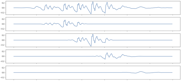
Figure 1 shows a visualization of a signal and 4 consecutive overlapping windows. Note how the amplitude at the extremities of the windows are atenuated compared to the original signal.

How many blocks $n_b$ do we have? The index of the last sample in the last block $n_b$ is denoted by $n_w + (n_b - 1) \Delta$, which might not coincide with the last sample in the original signal. We can either pad the end of the signal with 0s or truncate the last sample of the signal. If we do the latter, then we’ll get:

We can implement these ideas in Python, remembering that we use 0-index arrays:

def create_overlapping_blocks(x, w, R = 0.5):
    n = len(x)
    nw = len(w)
    step = floor(nw * (1 - R))
    nb = floor((n - nw) / step) + 1

    B = np.zeros((nb, nw))

    for i in range(nb):
        offset = i * step
        B[i, :] = w * x[offset : nw + offset]

    return B

A given index $i$ from the input signal will show up in one or more blocks, and in each of them it will be multiplied by the corresponding weight. More precisely, if it belongs to block $j$, the weight $x_i$ was multiplied by is $w_{i - (j - 1) \Delta}$.

Let $S_i$ be the set of all block indices to which index $i$ belongs. The sum the weighted $x_i$ across all blocks it belongs is given by:

If we choose our weight function $w$ such that

Then we can recover the original signal from the invidual blocks by adding the right indices, which is the Add part of Overlap-Add.

We can write a function to perform this:

def add_overlapping_blocks(B, w, R = 0.5):
    [count, nw] = X.shape
    step = floor(nw * R)

    n = (count-1) * step + nw

    x = np.zeros((n, ))

    for i in range(count):
        offset = i * step
        x[offset : nw + offset] += B[i, :]

    return x

Hann Window

The Hann window, also known as raised cosine window is a function that satisfies the properties we described above. Wikipedia offers some insight into the choice of a Hann function [3]:

In between the extremes are moderate windows, such as Hamming and Hann. They are commonly used in narrowband applications, such as the spectrum of a telephone channel.

It’s available in scipy.signal. The first parameter is the size of the window in number of points, which will determine the size of the blocks as we saw above. The author in [1] uses a window corresponding to 30ms.

The second parameter is whether the window is symmetric (that is the weights form a “palindrome”) or periodic. The periodic window of size $n$ is the same as the symmetric of size $n + 1$ without the last point: hann(n, False) == hann(n + 1, True)[:-1].

I don’t understand the details, but a periodic window seems to work better when working with spectral analysis of the signal [4], which is what we’ll be doing by inferring the frequency of the resonance filter.

from scipy.signal.windows import hann

sym = False # periodic
hann(floor(0.03 * sample_rate), sym) # 30ms window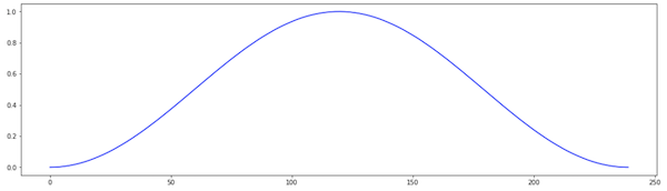

Encoding

We’ve seen how to massage the signal and break it into small chunks. Now we’ll see how to infer the coefficients from any given chunk using the source-filter model.

The LPC Model

Let $x_t$ be the amplitude of our signal at a given instant $t$. According to the source-filter model, it’s generated by a source signal $e$ going through a resonant filter $h$.

The $*$ denotes the convolution operator. The model further assumes that the current signal also depends on the past $p$ samples, that is $x_{t-1}, \cdots, x_{t-p}$, and that the source is constant, so effectively:

Solving the model

We then have $n - 1$ equations (one for each sample, except the first), and we have to determine the $p$ coefficients $\boldsymbol a = [a_1, \cdots, a_p]^T$ and $\boldsymbol e = [e_2, \cdots, e_n]$:

The approach taken in [1] is to ignore the errors and solve for $\boldsymbol a$, but trying to minimize the error. The error is then $\boldsymbol e$.

More precisely, we define the matrix $X$ where the $i$-th row is:

We assume that $x_i = 0$ if $i <= 0$. We define $b$ as the column vector: $[x_1, \cdots, x_n]^T$, and then w solve the linear system: $X \boldsymbol a = b$ for $\boldsymbol a$, minimizing the square of the error.

One way of constructing the matrix $X$ is to generate a vector $[x_n, x_{n-1}, \cdots, x_1, 0, \cdots, 0]$ and then assign the last $p$ entries to the first row ($[x_1, 0, \cdots, 0]$), then shift the window by one and assign to the second row ($[x_2, x_1, 0, \cdots, 0]$), and so on.

def make_matrix_X(x, p):
    n = len(x)
    # [x_n, ..., x_1, 0, ..., 0]
    xz = np.concatenate([x[::-1], np.zeros(p)])

    X = np.zeros((n - 1, p))
    for i in range(n - 1):
        offset = n - 1 - i
        X[i, :] = xz[offset : offset + p]
    return X

We can then use np.linalg.lstsq() to solve and find a:

def solve_lpc(x, p, ii):
    b = x[1:]

    X = make_matrix_X(x, p)

    a = np.linalg.lstsq(X, b.T)[0]

    e = b - np.dot(X, a)
    g = np.var(e)

    return [a, g]

The vector e is assumed to be samples from a white noise source. This can be modeled by a normal distribution with zero mean and the same variance $g = \sigma^2$, so this is the only parameter we need to store in our model.

Encoding the Whole Signal

We can now define the LPC algorithm, by first splitting the original signal into chunks then solving the model for each chunk:

def lpc_encode(x, p, w):
    B = create_overlapping_blocks(x, w)
    [nb, nw] = B.shape

    A = np.zeros((p, nb))
    G = np.zeros((1, nb))

    for i in range(nb):
        [a, g] = solve_lpc(B[i, :], p, i)

        A[:, i] = a
        G[:, i] = g

    return [A, G]

Decoding

Let’s look at recovering the signal from the coefficients obtained for any given chunk.

Simulating a Source-Filter Model

Decoding a LPC model consists in simulating a Source-Filter model: we first generate a source signal (white noise) and then apply a filter corresponding to the coefficients.

For the white noise, we get samples from a normal distribution. The function randn() implements a normal distribution with mean 0 and variance 1. To get a variance of g, we need to multiply by $\sqrt{g}$, since

I don’t know anything about digital filters (EDIT: this makes a lot more sense after Z-transform) but for now we can assume lfilter() is filtering a source signal (third argument) and amplifying certain frequencies specified by the coefficients in a (second argument).

def run_source_filter(a, g, block_size):
    src = np.sqrt(g)*randn(block_size, 1) # noise

    b = np.concatenate([np.array([-1]), a])

    x_hat = lfilter([1], b.T, src.T).T

    # convert Nx1 matrix into a N vector
    return np.squeeze(x_hat)

Decoding the Whole Signal

Now that we can decode the signal from a given single LPC model, we can generate all OLA blocks ($\hat B$) and add them back up to obtain the full signal ($\hat x$):

def lpc_decode(A, G, w, lowcut = 0):

    [ne, n] = G.shape
    nw = len(w)
    [p, _] = A.shape

    B_hat = np.zeros((n, nw))

    for i in range(n):
        B_hat[i,:] = run_source_filter(A[:, i], G[:, i], nw)

    # recover signal from blocks
    x_hat = add_overlapping_blocks(B_hat);

    return x_hat

One major difference from [1] is that they re-apply the window over the decode signal, that is,

B_hat[i,:] = np.multiply(w.T, B_hat[i,:])

My understanding is that we already applied these weights in add_overlapping_blocks() when generating the blocks, before encoding, so when we decode the signal would already be weighted.

Skipping this step didn’t seem to yield any difference in the output.

Experiment

We’ve defined all the building blocks, so we’re now ready to define our experiment by putting them all together.

Putting it all together

[sample_rate, amplitudes] = scipy.io.wavfile.read('lpc/audio/speech.wav')
amplitudes = np.array(amplitudes)

# normalize
amplitudes = 0.9*amplitudes/max(abs(amplitudes));

# resampling to 8kHz
target_sample_rate = 8000
target_size = int(len(amplitudes)*target_sample_rate/sample_rate)
amplitudes = resample(amplitudes, target_size)
sample_rate = target_sample_rate

# 30ms Hann window
sym = False # periodic
w = hann(floor(0.03*sample_rate), sym)

# Encode
p = 6 # number of poles
[A, G] = lpc_encode(amplitudes, p, w)

# Print stats
original_size = len(amplitudes)
model_size = A.size + G.size
print('Original signal size:', original_size)
print('Encoded signal size:', model_size)
print('Data reduction:', original_size/model_size)

xhat = lpc_decode(A, G, w)

scipy.io.wavfile.write("example.wav", sample_rate, xhat)
print('done')

The full code is available as a Jupyter notebook.

Results

Running with the audio speech.wav provided by [1], we obtained

Original signal size: 96,249 (floats)
Encoded signal size: 5,607 (floats)
Data reduction: 17x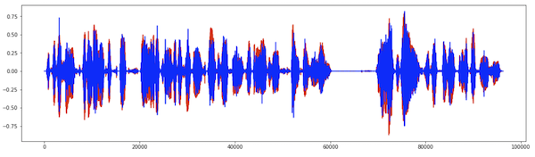

Conclusion

In this post we learned how to implement the LPC method for encoding and decoding in Python. As always, having to implement an algorithm made me understand it in much more depth, including the source-filter model.

This is the first time I deal with signal processing and there was a lot of concepts to learn. Hopefully my newbie perspective is helpful to other people starting on this area without formal training.

Digital filters seem like a vast area and something I’m interested in digging into [5].

Appendix: Converting Matlab to Python

I struggled a lot to make the Python code work, even when I had a working version of the Matlab code running throught Octave.

In dealing with multi-dimensional numerical applications like this, it’s very easy to get dimensions wrong because the APIs sometimes are permissive and do different things depending on the dimensions of the data we pass in. It is hard to validate intermediate results because they might not have a clear interpretation, making it harder to debug.

A few techniques were extremely helpful for debugging, leveraging the fact I had the Octave code. The idea is to compare intermediate results.

CSV exports/import. Due to differences in implementation and random number generation, it’s impossible to compare values - one idea is to save intermediate results into a CSV file from Octave then load into Python. If this happens inside a loop we pick a specific index.

Histogram of the data. A simpler technique, especially if there are no randomness involved is to display a histogram of the values in the matrix in both Python and Octave:

print('x', np.histogram(x.flatten()))

Numpy and Octave use the same number of buckets by default but choose the bucket label differently. It’s still useful for checking the number of elements in each bucket.

Visualizing. Another way to compare results is to plot the data in a timeseries. Even when randomness is involved the overall shape between Python and Octave should resemble each other.

Related Posts

Levinson Recursion - The whole reason we studied the Levinson Recursion algorithm is for the Linear Predicitve Coding algorithm. The matrix returned by make_matrix_X() is a Toeplitz once, but it’s not a square one. I haven’t found references on how to adapt the Levinson algorithm for non-square matrices.

References

• [1] Linear Predictive Coding is All-Pole Resonance Modeling - Hyung-Suk Kim
• [2] Signal Processing: Why is telephone audio sampled at 8 kHz?
• [3] Wikipedia: Window Functions, Comparison of windows
• [4] MathWorks - What is the ‘periodic’ sampling option in the HAMMING function?
• [5] Digital Filters

Source code | RSS feed | Tags: signal processing python