kuniga.me > NP-Incompleteness > CPU Cache
CPU Cache
24 Apr 2020
In this post we’ll study CPU caches. We’ll first understand why it exists, some of its typical properties and then explore vulnerabilities associated with CPU cache.
Motivation
According to Wikipedia [1]:
Microprocessors have advanced much faster than memory, especially in terms of their operating frequency, so memory became a performance bottleneck. How much faster is it? Doing some estimates based on a benchmark for Intel’s Haswell architecture [6], it seems that the worst case of RAM access is 100x slower than the fastest CPU cache. See Appendix A for how our calculations.
CPU cache is cache
I wanted to begin with this tautology to call out that many of properties and design of a high-level caching system we might be more familiar with also applies to a CPU cache. It was useful for me to keep this in mind for understanding this new topic.
For example, as we’ll see later in more details, a CPU cache can be seen as a key-value table, which requires hash-like strategies for assigning keys to rows and for cache eviction.
Types
There are multiple CPU caches and they perform different functions. It varies depending on the CPU model but there are some general similarities.
Hierarchy
The CPU cache is divided into multiple levels of cache. The first level, referred to as L1 is the fastest and smallest. The n-th level, Ln is the largest and slowest. Typical values of n seem to be 3 or 4. In a multi-core CPU, the first levels of cache are exclusive to each CPU, while the later levels are shared.
For a real-world example, Wikipedia [4] describes the architecture for Intel’s Kaby Lake architecture, where L1 is 64KB, L2 is 256KB and L3 is between 2MB to 8MB and shared by the cores.
Why do we have multiple-level of caches vs. a single level? This Q&A [5] suggests that it allows working with different tradeoffs of physical constraints, namely location and size of the component.
Data, Instruction, Address
L1 is often divided between data and instruction. As the name suggests, the L1-data caches data from memory needed during a program execution, while the L1-instruction caches the instructions needed to execute the program itself.
There’s another specialized cache called translation lookaside buffer, or TLB, which is used to lookup memory addresses (we’ll see more details later).
Why do we need separate caches for these 3 different uses? Wikipedia [1] provides an insight:
Pipelined CPUs access memory from multiple points in the pipeline: instruction fetch, virtual-to-physical address translation, and data fetch. The natural design is to use different physical caches for each of these points, so that no one physical resource has to be scheduled to service two points in the pipeline.
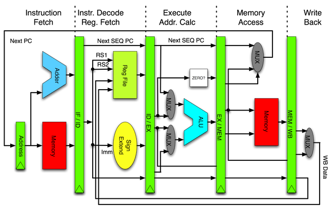
It’s worth recalling that a CPU operates in cycles and it follows a set of operations in a pipeline fashion (think of a conveyor belt in a factory). The following is a diagram of a possible CPU pipeline:
Structure
We’ll now analyze the structure of a CPU cache, in particular a data cache. Like any general purpose cache, it conceptually represents a lookup table or a key-value structure, so we’ll use this as our analogy to make absorbing new terminology easier.
Cache entry
We can think of the CPU cache as a table. If has n rows and m columns (Intel uses n = 64 and m = 8). A cell in this table is called a cache line and it has a fixed size k bytes (Intel uses k = 64). The row of the table is also known as index.
Storing. Suppose we want to cache an object currently in the RAM and of size 32 bits, located at the address A, so we need to cache the segment [A, A + 4) (recalling that addresses points to bytes, that is there’s 8-bits between A and A + 1).
Now, the important thing to observe is that an entire block is moved to the cache line, not just the segment [A, A + 4). Suppose the cache line is 64 bytes. To find to which 64-block A belongs, we can set its 6 least significant bits to 0, which we call A'. Then the whole block [A', A' + 6) will be stored in the cache line.
It’s entirely possible that the object crosses the block boundary, that is A + 4 > A' + 6, in which case the next block [A' + 6, A' + 12) would need to be stored as well, in a different cache line.
To determine the index or row in which to store the cache line we use the next bits of the address. Assuming n = 64 = 2^6, we can use the next 6-bits (b[6..12]) to determine the index. Once the index is found, we need to determine which of the m columns to store the cache line in, which we’ll discuss next.
We also need to store the remaining 64 - 6*2 = 52 bits alongside the data to validate the data cache is the correct one upon reading (due to collisions). This is called the tag.
Reading. To determine whether an address is in the cache, we use the same bits b[6..12] to find the correct index. Then we need to compute the tag from the bits b[12..64] and look for a column that contains the same tag.
Associativity
In the process above, we may have collisions because any addresses that have the same bits b[6..12] will be mapped to the same index.
On one side a CPU cache is “bare metal” hardware, so complex hash collision resolution strategies is infeasible to implement. On the other hand it is a cache, not a persistent key-value store, meaning that when a collision happen we can just evict the previous entry.
Still, high eviction rates can also mean high cache misses rates which is a key quality factor of a cache. Given the limited size of a cache, there are two dimensions we can tradeoff: number of indexes and number of cache entries per index. In our analogy with hash tables, this would roughly map to number of entries vs. max number of collisions supported.
Some common strategies are either having m = 1 (direct mapping), m = 2 (two-way set associativity) or some higher number like Intel’s m = 8 [6]. Any such strategy is what we call associativity. Let’s take a closer look at these strategies.
A group of cache lines within the same index is called a set.
Direct-mapping. Like a hash table with a simple function. Each set has exactly one cache line. If a new entry maps to a row already “occupied”, the previous entry is evicted.
The advantage of this is simplicity: there’s no criteria we need to use to choose which “cell” of our table to assign it to once we determined its row, since there’s only one. Eviction is easy too.
The downside is that we’re subject of degenerate cases where two hot addresses map to the same index. This will result in the entries being swapped out and many cache misses.
Two-way set associativity. In this case, each set has 2 cache lines, so a given memory address can go to any of the two. When deciding which cache line to assign it to, we can use LRU (least recently used).
To do so, we need an extra bit to keep track of this information: every time a cache line is read, we set a bit in it to 1 and to 0 in the other. On writes, we can always evict the slot with bit 0.
This is a more complex approach than direct-mapping and we need to use a bit to keep account for the LRU. On the other hand it avoids the degenerate case of a direct-mapping, but suffers the same if there are 3 or more hot addresses.
m-way associative cache. A more general structure would be m cache lines per set. This further shifts the balance between complexity (the higher the m the more expensive it is) and avoiding degenerate cases (resilient to up N hot addresses).
Concurrency
When the CPU performs some computation, it might write to its L1 cache before it syncs with the RAM (write-back caching). When it does that, it marks the corresponding cache line as dirty by setting a bit, and eventually this data is written back to the RAM.
The picture gets complicated in multi-processor systems. As we discussed before, each CPU has its own L1 cache. However, it’s possible that the same region of RAM is in the L1 cache of multiple CPUs.
CPUs cannot leverage read and write locks because they’re too expensive at the CPU level. To support sharing cache lines, the CPUs must follow some protocol, such as the MESI protocol. These protocols are called cache coherence protocols.
The protocol name stands for the possible states a cache line at each CPU might be in: Modified, Exclusive, Shared and Invalid (at any given time the same cache line can have different states for different CPUs).
- Modified: this means this CPU has exclusive access to the cache line and it has local modifications (dirty)
- Exclusive: this means this CPU has exclusive access to the cache line but it’s clean
- Shared: other CPUs may also have this cache line and it’s clean
- Invalid: this CPU has the cache line but it cannot read or write to it.
The protocol dictates that, for example, if one CPU has a cache line in the “modified” state, then if any other CPU has the same cache line, it must be in the “invalid” state.
If CPU 1 wants to write to a cache line, it must first inform the other CPUs to invalidate their copies (i.e. set them to the “invalid” state). If one of those CPUs has a cache line in the “modified” state, the changes must be flushed to RAM.
If later another CPU 2 needs to write to that cache line, it first needs to tell CPU 1 to flush its modifications and set its state to “invalid”. Then CPU 2 has to re-populate its cache line from memory.
This can keep going on back-and-forth, leading to an issue called cache line bouncing.
Translation Lookaside Buffer
Before we describe the translation lookaside buffer, we need to revisit virtual memory.
Virtual Memory: a prelude
Virtual memory is an abstraction layer that hides the details of physical memory. Some use cases:
- Memory is fragmented in the physical space but is contiguous in the virtual space. Storage is made transparent to programs - the OS can decide whether to store data in memory or in disk.
- Programs can have their own (virtual) address space. For example, both programs A and B could access their own address X and not have conflict, since these are mapped to different physical addresses. Virtual memory is chunked in blocks of fixed size which are called (virtual) pages. The page size is defined by the processor (mine in 4KiB). The corresponding physical page is called page frame [3].
The mapping between virtual memory and physical memory is done by the memory management unit, or MMU. It keeps a table (page table) in memory (RAM) that has one entry for each page and it maps to corresponding the physical address.
Why memory is segmented in pages? The page table is a likely reason. If we mapped byte to byte, then the page table wouldn’t fit in memory because we’d need an entry for every byte! We need a good balance between a page that’s not too big (coarse granularity) which would lead to wasted memory if most of the page went unused vs. a page that’s not too small (fine granularity) which would lead to a gigantic page table.
TLB: The page table cache
Many of CPU instructions require access to data in (physical) memory, so it needs to translate a given virtual address to its physical correspondent. As we’ve seen, memory access is slow, so not surprisingly there’s also a cache for the page table, which is called translation lookaside buffer (TLB).
Page or Cache Coloring
Imagine our application needs access to a large block of memory - this will consist of a list of virtual pages that are adjacent in the virtual address space. However, these are not guaranteed to be adjacent in the physical address space.
The CPU cache is designed to map adjacent physical addresses to different cache lines. This is so that accessing a contiguous piece of physical memory will enable most of the data will be on cache at a time. If they mapped to the same cache line, we’d evict.
What can happen is that a list of adjacent virtual pages are not physically adjacent, which means there’s no guarantee they will map to different cache lines.
To address this problem, pages frames are “colored” based on which cache line they would be assigned to [8]. The corresponding virtual page “inherits” that color. When assigning sequential pages to physical locations, the OS tries to make sure that contiguous pages will have a diverse set of colors.
Security
Whenever adding caching to improve the performance of a system, an important consideration is security. One example could be caching some expensive computation which also perform access checks. The cached data could be vulnerable if an attacker has access to the key.
We’ll now concentrate into two famous exploits known as Spectre and Meltdown. Before that, we need to understand out of order execution.
Out of order execution
In conjunction with caching, an optimization technique the CPU employs to speed up execution is to execute instructions ahead of time (out of order) if it can guarantee the end result is correct.
For example, say one instruction i requires reading from a value from memory, which can be expensive on a cache miss. Say that the next instruction i+1 doesn’t depend on this value. The CPU can then execute that instruction i+1 before i is finished.
One more concrete example is called branch prediction. Say your code has a conditional like:
if (condition) {
expression1;
} else {
expression2;
}
and that evaluating condition is slow. Then the CPU might predict condition=true and execute expression1 before it knows whether condition is true. If it happens to be false, it just resumes the execution at the other branch.
Meltdown and Spectre
A few years ago, two vulnerabilities were found related to CPU cache, named Spectre and Meltdown. Let’s analyze the Spectre [11] first.
Spectre.
As we mentioned above, the CPU might perform branch prediction. The problem with that is the CPU will cache the result of expression1 even if it turns out to be abandoned later.
Consider the following contrived example proposed by ricbit [7]:
if (bigvalue < a.length) {
  value = a[bigvalue];
  if (value & 1 > 0) {
    x = a[100];
  } else {
    x = a[200];
  }
}
// Timing attack
const t1 = performance.now();
const y1 = a[100];
const duration1 = performance.now() - t1;

const t2 = performance.now();
const y2 = a[200];
const duration2 = performance.now() - t2;

if (duration1 * 10 < duration2) {
  // a[100] is cached, value & 1 = 1
} else if (duration2 * 10 < duration1) {
  // a[200] is cached, value & 1 = 0
}
Suppose we want to read the contents of the memory address represented by
a[bigvalue]
Because we didn’t explicitly allocate memory for that position, we’ll generally not have access to that. But say we can be sure the CPU will perform branch prediction in
bigvalue < a.length

And predict it will be true. Then it will execute the next few lines before it determines the condition is actually false. By that time it accessed the value in a[bigvalue] without permission checks. If the last bit of the value is 1, xwill have the value of a[100] and but importantly the CPU will cache the memory address represented by a[100]. Otherwise, it will do the same with a[200].
After the branch prediction fails and it’s cleaned up, we execute our timing attack. It simply measure the time to access both a[100] and a[200]. Whichever address is cached will return much faster, which in turn is a proxy for the last bit of the value in a[bigvalue]. Repeat this will all the bits and we’ll get the exact value.
Meltdown
Meltdown uses a similar approach [12], but instead of relying on branch prediction, it relies on CPU executing instructions after an exception is raised, so if the application manages to handle the exception, it can then use timing attacks to detect what value was cached.
The paper provides a code in assembly. I’ve attempted to write a pseudo (meaning it doesn’t work but captures the idea of the exploit) version in C for educational purposes:
#include <setjmp.h>
#include <signal.h>
#include <stdio.h>
#include <string.h>

void primer(char probe[256]) {
    // Some specific address
    int addr = 136322;
    // This will throw segmentation fault, but we're "catching it"
    char v = *(char *)addr;
    // This will be executed spectulatively by the CPU
    probe[v] = 1;
}

sigjmp_buf point;

// segfault signal handling
static void handler(int sig, siginfo_t *dont_care, void *dont_care_either) {
   longjmp(point, 1);
}

int main() {
    struct sigaction sa;
    memset(&sa, 0, sizeof(sigaction));
    sigemptyset(&sa.sa_mask);

    sa.sa_flags     = SA_NODEFER;
    sa.sa_sigaction = handler;
    sigaction(SIGSEGV, &sa, NULL);

    char probe[256];
    if (setjmp(point) == 0) {
        primer(probe);
    } else {
        printf("Read chunks of probe and check which one is cached\n");
    }

    return 0;
}
The steps are:

1-) Try accessing some protected memory address but exception is thrown due to invalid access. But handle the exception so that application doesn’t crash.
2-) Right after the exception, use the content of the protected address as index of a probe array (non-protected address). This exploits a CPU behavior that executes instructions out-of-order and caching them. In this scenario, it will execute the instruction above and cache that portion of the array.
3-) Timing: Try reading parts of the array and measure which one returns faster, indicating that address is cached, and hence we know that that address
Spectre vs. Meltdown?
One of the most difficult things for me is to understand the precise difference between Spectre and Meltdown. I’ve seen a lot of comparisons between the 2, but they’re too high-level to satisfy my curiosity. On the other hand the distinction provided by the papers are hard for me to grasp.
The discussion of Spectre [11] on Meltdown is a bit clearer:
Meltdown is a related attack which exploits out-of-order execution to leak kernel memory. Meltdown is distinct from Spectre attacks in two main ways. First, unlike Spectre, Meltdown does not use branch prediction. Instead, it relies on the observation that when an instruction causes a trap, following instructions are executed out-oforder before being terminated. Second, Meltdown exploits a vulnerability specific to many Intel and some ARM processors which allows certain speculatively executed instructions to bypass memory protection. Combining these issues, Meltdown accesses kernel memory from user space. This access causes a trap, but before the trap is issued, the instructions that follow the access leak the contents of the accessed memory through a cache covert channel.
The remarks of Meltdown [12] on Spectre in more succinct and obscure:
Meltdown is distinct from the Spectre Attacks in several ways, notably that Spectre requires tailoring to the victim process’s software environment, but applies more broadly to CPUs. My feeling is that the differences are too specific and technical to be explained in a simple way, yet I seem to lack the background to understand them fully.
Conclusion
I was reading a paper that made references to CPU cache cache lines, so that prompted me to research about it. I was surprised to learn how much information there is about it, so decided to dedicate an entire post for it.
It was also great to dive deeper in understanding about Spectre and Meltdown, even though I didn’t fully internalize their specifics. I also learned a lot about virtual memory.
Appendix A: RAM vs Cache latency estimates
[6] provides a benchmark for Intel’s Haswell architecture, a high-end i7-4770. It provides data in terms of CPU cycles:
- L1: 4-5 cycles
- L2: 12 cycles
- L3: 36-58 cycles
- RAM: 36 cycles + 57ns / 62 cycles + 100 ns We can see that L3 can be roughly 10x slower than L1. To compare apples to apples, we need to convert cycles to time so we can add the overhead from the RAM. The CPU in question operates at 3.4GHz, which means a cycle is about 0.294ns. So 4 cycles of L1 takes abount 1.17ns and the worst case for RAM of 62 cycles + 100 ns is about 118ns, which gives us 100x slower latency estimate.
Related Posts
- Von Neumann Architecture - We presented an overview of the architecture many computers use. We briefly touched on memory bottlenecks and CPU cache.
- Content Delivery Network - As discussed, CDN is another kind of cache, that lives in a much much higher level of the stack.
- Python Coroutines - Not directly related to caching, but the out-of-order execution reminds me a lot of the co-routine execution. One task waiting on I/O might get queued for later the same way an instruction waiting for - an expensive - memory read is queued.
- Browser Performance - This is relevant to timing attacks - memory access is relatively slow, but still very fast in absolute terms. The Appendix A above calculates the latency on the order of 100ns. To be able to determine if the data was cached, the measurement has to have high-precision. To help reducing this vulnerability, browser purposefully reduce the precision of APIs such
performance.now().
Mentioned by Buddy Memory Allocation.
References
- [1] Wikipedia - CPU cache
- [2] Wikipedia - Virtual memory
- [3] What is the difference between a ‘page’ of memory and a ‘frame’ of memory?
- [4] Wikipedia - Cache hierarchy
- [5] Why do we need multiple levels of cache memory?
- [6] 7-Zip LZMA Benchmark - Haswell
- [7] Ricbit Permanente - 2018/01/04 (in Portuguese)
- [8] Wikipedia - Cache Coloring
- [9] kunigami.blog - Content Delivery Network
- [10] Meltdown and Spectre
- [11] Spectre Attacks: Exploiting Speculative Execution - Kocher et al.
- [12] Meltdown: Reading Kernel Memory from User Space - Lipp et al.
