kuniga.me > NP-Incompleteness > Euclidean Minimum Spanning Tree
Euclidean Minimum Spanning Tree
17 Aug 2026
Otakar Borůvka was a Czech mathematician who is best known for his work in graph theory. Once, his friend Jindřich Saxel, an employee of the West Moravian Power Company, asked him for help optimizing electric distribution networks.
Borůvka modeled the problem as the minimum spanning tree problem and then came up with the first known algorithm to solve it, now known as the Borůvka algorithm.
In this post we’ll explore the Borůvka algorithm combined with KD-trees to solve the Euclidean Minimum Spanning Tree problem more efficiently.
Problem
The Euclidean Minimum Spanning Tree problem (EMST) consists in finding the minimum spanning tree (MST) of a set of $N$ points in the Euclidean space.
Algorithms such as Kruskal can find the MST of a graph $G(V, E)$ in $O(\abs{E} \log \abs{E})$. However in EMST the edges are implicit. The graph is a complete one where the weight of the edge between two points is their Euclidean distance, so a naive implementation consisting in computing the edges explicitly leads to a $O(N^2 \log N)$ algorithm.
Solution
In this post we’ll explore a more efficient implementation using the Borůvka algorithm with KD-trees which runs closer to $O(N \log^2 N)$ on average, even though the worst case is $O(N^2 \log N)$.
We’ll start by describing the Borůvka Algorithm to compute the MST. Note that there’s nothing special about it with respect to the Euclidean variant. It’s just that it operates in batches and we can leverage that to search on the KD-trees more efficiently.
Borůvka Algorithm
Interestingly enough, the problem that motivated the Borůvka algorithm can be modeled as a Euclidean graph, where vertices are cities and edges between them have costs corresponding to the Euclidean distance. However his algorithm works on general graphs and doesn’t exploit the Euclidean properties.
Like Kruskal and Prim, the Borůvka algorithm is greedy, at each step taking the optimal decision and that leads to the optimal solution. In high level terms:
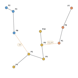
At start, each vertex belongs to its own component. Then we loop until one component remains:
- For each component, select the cheapest edge to another component. Collect all these edges first.
- For each edge:
- If they connect two components, merge them into one, add the edge to the solution.
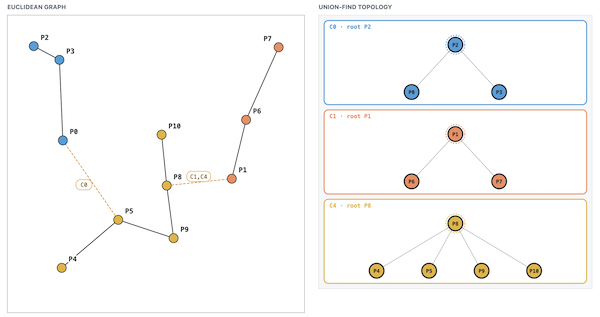
This algorithm feels like a fusion between Kruskal (add cheapest edges to the MST) and Prim (grow a component). I guess it’s not as popular as either because the implementation is less simple. The steps are very suggestive of the union-find data structure and indeed it’s used in the implementation.
First, let’s prove the correctness of this algorithm: the idea is that at any point in time, the solution contains a subset of a MST (Lemma 1). This then implies the edges in the solution form a forest (i.e. each component is a tree). Since only one component is left at the end, it must be a tree and hence a MST.
Lemma 1. At each step of the iteration of the Borůvka algorithm the set of selected edges is a subset of the edges of some spanning tree of minimum cost.
Otherwise assume no MST contains $E \cup \curly{e}$. Since $A$ must be connected to the rest of the forest at some point, there's an edge $f$ leaving $A$ such that $E \cup \curly{f}$ is in some MST $T$. If we remove $f$, we're left with two components, $A$ and $V \setminus A$. By construction $e$ is also an edge from $A$ to $V \setminus A$, so we can replace $f$ with $e$ on the MST. By construction $w_{e} \le w_{f}$. If $w_e = w_f$ then we have another MST containing $E \cup \curly{e}$, but that's a contradiction. If $w_{e} \lt w_{f}$, then we found a new spanning tree with smaller cost, so $T$ is not a MST.
The simplest way to implement this algorithm is to keep a list of all candidate edges. Then at the beginning of the iteration, keep only edges that are across components (using union-find) and then for each component, track the cheapest edge. We can determine whether two vertices are in the same component of a union find in $O(1)$ amortized, and also merge two components in $O(1)$. This makes each iteration $O(\abs{E})$.
At each iteration, each component will be merged into some other component, so the number of components will at least halve. Thus there are only $O(\log \abs{V})$ iterations leading to a $O(\abs{E} \log \abs{V})$ algorithm.
Implementation
As discussed above, the algorithm uses the union find data structure, which we’ll implement using UnionFind. The implementation details are collapsed below. We just need to understand the methods: .find(x) -> int which returns the component of a given member x, and .union(x, y) which merges the components of x and y.
class UnionFind:
    def __init__(self, n):
        self.p = list(range(n))
        self.s = [1]*n
        self.sz = n

    def find(self, x):
        p = self.p
        if p[x] != x:
            p[x] = self.find(p[x])
        return p[x]

    def union(self, x, y):
        px, py = self.find(x), self.find(y)
        if px == py:
            return

        s, p = self.s, self.p
        if s[px] < s[py]:
            px, py = py, px

        s[px] += s[py]
        p[py] = p[px]

        self.sz -= 1
        return s[px]

    def size(self):
        return self.sz
We also define a few utility classes to help with syntax, but their meaning is intuitive, for example Point and BoundingBox. A bounding box is the smallest axis-aligned box containing a set of points. We represent it by its “lower” and “upper” corners.
def norm_sq(p) -> float:
    return sum(x*x for x in p)

@dataclass(frozen=True)
class Point:
    data: tuple[int, ...]

    def __getitem__(self, dim: Dimension):
        return self.data[dim.v]

    def __len__(self) -> int:
        return len(self.data)

    def __abs__(self) -> float:
        return sqrt(norm_sq(self))

    def __sub__(self, other: Point):
        sub = tuple(a-b for a,b in zip(self.data, other.data))
        return Point(sub)

    def __iter__(self):
          return iter(self.data)

@dataclass
class BoundingBox:
    lo: Point
    hi: Point

    @staticmethod
    def for_point(p):
        return BoundingBox(p, p)

    def union(self, bb):
        if bb is None:
            return self

        self.lo =  Point(
            tuple(min(px, qx) for (px, qx) in zip(self.lo, bb.lo))
        )
        self.hi =  Point(
            tuple(max(px, qx) for (px, qx) in zip(self.hi, bb.hi))
        )

    def size(self):
        'Square length of the diagonal'
        return norm_sq(self.lo - self.hi)
We can start defining an interface for any algorithms computing the Euclidean minimum spanning tree from a set of points:
class EMST(ABC):
    @abstractmethod
    def desc(self) -> str:
        "Describe the algorithm"

    @abstractmethod
    def get_mst_edges(self, points: list[Point]) -> list[Edge]:
        pass
And then define the specialization for Borůvka:
class Boruvka(EMST):
    def setup(self, points: list[Point]):
        pass

    @abstractmethod
    def fill_best_edge_by_component():
        pass

    def get_mst_edges(self, points: list[Point]) -> list[Edge]:
        n = len(points)
        uf = UnionFind(n)
        self._uf = uf

        self.setup(points)

        sol = []
        while uf.size() > 1:
            self._best_edges = {}
            self.fill_best_edge_by_component()
            for e in self._best_edges.values():
                uc, vc, _ = e
                if self.merge_components(uc, vc):
                    sol.append(e)
        return sol
The core of this algorithm is fill_best_edge_by_component(), i.e. for each component in the union-find, determine the shortest edge from it to some other component. From there we determine which edges to keep and which components to merge.
We also add some helper functions that are used by different Borůvka implementations, mostly to avoid repeated code when dealing with the union find structure such as merge_components() and process_edge() (see if it’s worth adding an edge to the best edge by component).
class Boruvka(EMST):
    ...
    # Helper methods

    def merge_components(self, p, q) -> bool:
        'Combine components of p and q into one'
        if self._uf.find(p) == self._uf.find(q):
            return False
        self._uf.union(p, q)
        return True

    def get_component(self, p):
        return self._uf.find(p)

    def get_best_dist(self, p):
        pc = self.get_component(p)
        if pc not in self._best_edges:
            return inf
        return self._best_edges[pc][2]

    def process_edge_for_component(self, c, e):
        _, _, w = e
        if self.get_best_dist(c) > w:
            self._best_edges[c] = e

    def process_edge(self, e):
        u, v, w = e
        uc, vc = self.get_component(u), self.get_component(v)
        if uc == vc:
            return

        self.process_edge_for_component(uc, e)
        self.process_edge_for_component(vc, e)
Now we are ready for our first implementation of the “naïve” Borůvka, one where we compute the set of edges explicitly. With the helpers we defined, the code is straightforward: to compute the best edge set, we just process each of the $O(N^2)$ edges one at a time:
class NaiveBoruvka(Boruvka):
    def desc(self) -> str:
        return "Naive Boruvka"

    def setup(self, points: list[Point]):
        n = len(points)
        edges = []
        for i in range(n):
            for j in range(i + 1, n):
                edges.append((i, j, dist(points[i], points[j])))
        self._edges = edges


    def fill_best_edge_by_component(self):
        for e in self._edges:
            self.process_edge(e)
KD-Tree
In KD-Tree we learned that this binary structure allows us to search for the nearest point by splitting clusters of points into different subtrees.
It works well in practice, closer to $O(\log N)$ search, even though in the worst case it’s $O(N)$. We can use it to find the closest point $p$ to each point $q$ so that the edges $(p, q)$ are the only ones that need to be accounted for. Conceptually we could implement fill_best_edge_by_component() as:
class KDTreeBoruvka(Boruvka):
  ...
  def fill_best_edge_by_component(self):
      for q in points:
          p = self.get_closest_point(kd, q)
          self.process_edge((q, p, dist(p, q)))
Since on average we expect each search to be $O(\log N)$, fill_best_edge_by_component() is $O(N \log N)$ and the Borůvka becomes $O(N \log^2 N)$.
We can’t use a generic search for kd-tree because now we need to account for the components of the points: Points on the same component are not candidates for closest neighbors. The difference with query_kd_tree() in the original implementation is quite small though.
class KDTreeBoruvka(KDTreeBoruvkaBased):
    def desc(self) -> str:
        return "KD-Tree Boruvka"

    def setup(self, points: list[Point]):
        n = len(points)
        view = View(points)
        self._kd = build_kd_tree(view, Dimension(n=3))
        self._points = points

    def query_kd_tree(self, node, q, dim):
        if not node:
            return

        p = node.pivot
        Q, P = self.get_point(q), self.get_point(p)

        self.process_edge((q, p, dist(Q, P)))

        if node.is_leaf():
            return

        if Q[dim] <= P[dim]:
            main = node.left
            other = node.right
        else:
            main = node.right
            other = node.left

        self.query_kd_tree(main, q, dim.next())

        if other:
            lb = abs(Q[dim] - P[dim])
            ub = self.get_best_dist(q)
            if lb < ub:
                # needs to search in the other tree
                self.query_kd_tree(other, q, dim.next())

    def fill_best_edge_by_component(self):
        for i in range(len(self._points)):
            self.query_kd_tree(self._kd, i, Dimension(n=3))
Here, when comparing the query point q with a candidate (node.pivot), we call self.process_edge() which should ignore edges from points on the same component. We also work with indices of points instead of the points directly because we need the indices to do the union find properly. Other than that it’s exactly the same idea.
Optimizations
There are several optimizations we can do such as:
1-) Keep a bounding box for each node, so that instead of calculating the lower bound as the distance to the pivot line:
lb = abs(Q[dim] - P[dim])We can do it to the bounding box of that subtree, which is tighter:
lb = point_box_distance(Q, other.bb)2-) Store the set of the component ids in each subtree. If there’s only one and it’s the same as the query point, the entire search can be short-circuited.
This approach requires re-calculation after each iteration because the components change after merge but it’s a $O(N)$ step and the iteration is dominated by $O(N \log N)$ anyway. Then we can add this check in query_kd_tree():
class KDTreeBoruvka(KDTreeBoruvkaBased):
    def desc(self) -> str:
        return "KD-Tree Boruvka"

    def query_kd_tree(self, node, q, dim):
        if not node:
            return

        # prune: same component
        if node.components == {self.get_component(q)}:
            return

        ...
3-) A larger and more intrusive optimization is to not search the kd-tree for one point at a time, but instead traverse the kd-tree side by side and compute the distance for all points using a single traversal.
The algorithm is a lot more complicated and while my implementation of this version was 2x faster than the basic kd-tree one, it seems to be still a $O(N \log^2 N)$ process.
4-) Codex did a version with even more heuristics and optimizations, reaching a 4x speed up, but it removed a lot of the abstractions and the code became very hard to read, so I don’t think it’s very instructive.
The code for all these variants is on Github.
Experiments
During my experiments, I also used SciPy’s Minimum Spanning Tree algorithm, mostly to check correctness, but ended up including it in the benchmark as well. Since it’s so easy to translate code between languages, I asked Codex to convert its optimized Python implementation into C++ and Rust.
I ran these algorithms with sets of random points in 3D: $10^3$, $10^4$ and $10^5$ points. The runtimes in seconds are tabulated below:
| Algorithm | $10^3$ points | $10^4$ points | $10^5$ points |
|---|---|---|---|
| Naïve Borůvka | 1.35 | 182.63 | - |
| SciPy’s MST | 0.77 | 83.638 | - |
| KD-Tree Boruvka | 0.32 | 4.22 | 96.1 |
| KD-Tree Boruvka Dual | 0.15 | 2.32 | 26.66 |
| Optimized Python (Codex) | 0.08 | 1.31 | 36.63 |
| Naïve Borůvka C++ (Codex) | 0.005 | 0.47 | 37.61 |
| Optimized Rust (Codex) | 0.002 | 0.030 | 0.28 |
| Optimized C++ (Codex) | 0.003 | 0.036 | 0.31 |
We can see that C++/Rust are much faster than Python. The naive $O(N^2 \log N)$ C++ implementation is comparable to the optimized $O(N \log^2 N)$ ones even for $10^5$ and beats all the Python implementations for $10^4$.
Delaunay Triangulation
For the 2D case, a faster and simpler alternative exists, because it’s possible to show that the edges of a Euclidean MST of a set of points $P$ are a subset of the Delaunay triangulation of $P$.
The Delaunay triangulation of $N$ points in 2D has $O(N)$ edges and can be computed in $O(N \log N)$, so then running a regular $O(\abs{E} \log \abs{E})$ algorithm is very efficient. However for the 3D case, which is the case I was interested in, the number of edges can be $O(N^2)$.
So I studied Delaunay triangulation because I thought it was the best implementation for EMST but later I learned about the $O(N^2)$ edges.
Conclusion
This concludes a series of posts, which includes Delaunay triangulation, KD-trees and now the Borůvka algorithm.
It was motivated by a problem in Advent of Code which reduced to finding an EMST for 1,000 points in 3D. My Kruskal $O(N^2 \log N)$ ran in a few seconds but I wondered how much better it could be, so I went on this rabbit hole. Little did I know that if I had reimplemented Kruskal in C++, it would be faster than the Borůvka + KD-tree, but it’s never about the destination: I learned a lot during this process.
Related Posts
In An Introduction to Matroids we mentioned that the minimum/maximum spanning tree problem can be modeled as a matroid. Matroids can be solved by greedy polynomial-time algorithms and the Kruskal algorithm is the version that solves the matroid corresponding to MST. The Borůvka algorithm is also greedy.
There’s a generalization of the EMST called the Steiner Tree Problem, in which you can introduce intermediate nodes to try to reduce the cost of the solution, but solving this problem is NP-Complete.
The Steiner tree sounds a lot like the problem of Constructing Trees from a Distance Matrix which is also known as the tree metric realization problem, in which we can also introduce intermediate nodes, but in this case we’re deciding whether a tree can exist such that the distance between leaves (path length) matches a prescribed distance.