kuniga.me > NP-Incompleteness > Matroid Intersection
Matroid Intersection
13 Jan 2023
Stein Krogdahl was a Norwegian Computer Science professor at the University of Oslo. I couldn’t find much information about him on the web but his DBLP page shows an interesting history: Krogdahl seemed to have done research on theoretical computer science during his early career (70’s) before switching to to programming languages and software engineering research.
In particular, he wrote a single-author technical report on matroids, A Combinatorial Base for Some Optimal Matroid Intersection Algorithms [1], and then another single-author paper The dependence graph for bases in matroids. The TR is from Stanford, and mentions:
This work was supported in part by The Norwegian Research Council for Science and the Humanities.
The TR is dated to 1974 and Krogdahl seemed to be ~29 years old at the time, so one possibility is that he was a postdoc at Stanford, but it’s unclear who was he working with. In the TR, Krogdahl provides simpler proofs for results on matroid intersections originally introduced by Lawler:
E. Lawler has given an algorithm for finding maximum weight intersections for a pair of matroids (…)
And continues with the motivation:
However, the proofs given for the correctness of these algorithms have used linear programming concepts such as primal and dual solutions, and have been rather difficult to understand.
Lawler later uses Krogdahl proofs in his own Combinatorial Optimization: Networks and Matroids [2].
In this post we’ll study the problem of finding the largest independent set in the intersection of two matroids, known as the Matroid Intersection problem. We’ll be making use of the theorems and proofs from Krogdahl.
This is a continuation of my study on matroids and this post will rely on knowledge and definitions from Partition Matroids [3]. It’s also worth reading about the Hungarian Algorithm [4] since the algorithm for solving the Matroid Intersection problem borrows many ideas from it.
We’ll first state the problem more formally, build an intuition on the algorithm via augmenting sequences, define an auxiliary data structure called border graph and finally describe the algorithm and provide the implementation in Python.
Matroid Intersection Problem
Let $M_1(A, \cal I_1)$ and $M_2(A, \cal I_2)$ be two matroids over the same set $A$ but with (possibly) different family of independent sets $\cal I_1, \cal I_2$. We wish to find an independent set $I \in \cal I_1 \cap \cal I_2$ of maximum cardinality.
Intuition
The idea behind the matroid intersection algorithm is that we can improve on existing solutions by taking incremental steps greedly. Let’s build a sense of the algorithm via a concrete example (from [2]). Suppose we’re given graphs $G_1 = (V, E)$ and $G_2 = (V, E)$ as in Figure 1 and we want to find the largest subset of edges that do not form a cycle in either of them.
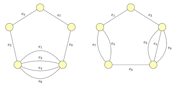
If we take the graphic matroids [2] $M_1 = (V, \cal I_1)$ and $M_2 = (V, \cal I_2)$ corresponding to graphs $G_1$ and $G_2$ respectively, then $I \in \cal I_1$ represents any subset of edges that are cycle free in $G_1$, and similarly for $I \in \cal I_2$. So the problem we’re trying to solve is finding the largest $I \in \cal I_1 \cap \cal I_2$.
Suppose we are given a valid solution $\curly{e_4, e_5}$ and we want to see if we can improve it. It’s easy to verify we cannot add any edge to it without creating a cycle in either $G_1$ or $G_2$.
Fortunately it’s still possible to greedly find a bigger subset from an existing one as long as it’s not already the maximum, by removing some edges and adding others, using an idea analogous to augmenting paths from bipatitie matching [4].
Augmenting Sequence I
Let’s get an intuition for an augmenting sequence in the matroid world via our example. First we try to add an edge not in $I = \curly{e_4, e_5}$ such that adding it to $I$ does not form a cycle in $G_1$. Suppose we choose $e_2$. It unfortunately forms the cycle $\curly{e_2, e_4}$ in $G_2$.
Now we need to choose an edge to break this cycle, but we can’t pick $e_2$ since it would take us back to the start. This only leaves $e_4$ as option. So our sequence is now $e_2, e_4$. We then try to find an edge such that adding it to $I + e_2 - e_4$ does not form a cycle in $G_1$. One such edge is $e_1$, so our sequence is $e_2, e_4, e_1$. It happens that $I + e_2 - e_4 + e_1 = \curly{e_1, e_2, e_5}$ also doesn’t form a cycle in $G_2$, so $e_2, e_4, e_1$ is an augmenting sequence. Figure 2 depicts this process.
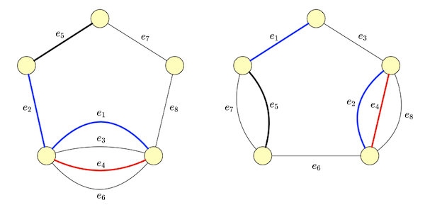
Adding and removing alternately the elements from the augmenting sequence to $I$ (i.e. add elements in odd positions and removing those in even positions), yields a larger set, much like “flipping” the edges in a augmenting path increases the match size by 1.
This analogy to augmenting paths in bipartite graphs can be taken further, but before we do that, let’s formalize these ideas and introduce some definitions.
Formalism
Let’s generalize the ideas above for graphic matroids by considering arbritary matroids $M_1(A, \cal I_1)$ and $M_2(A, \cal I_2)$.
Terminology
Let $M(A, \cal I)$ be a matroid and $B$ be a subset of $A$. The rank of $B$, denoted by $r(B)$, is the size of the largest independent set it contains. Note that if $B \in \cal I$, then $r(B) = \abs{B}$ and if $B = A$, then $r(B)$ is the size of the largest element in $\cal I$. For example, in $G_1$ above the subset $B = \curly{e_1, e_3, e_2}$ has rank 2, since $e_1$ and $e_3$ form a cycle and only $\curly{e_1, e_2}$ and $\curly{e_1, e_3}$ are independent sets.
A circuit is a minimal dependent set. That is, if we remove any element from it, the resulting set will belong to $\cal I$. To distinguish between circuits in the two matroids, we’ll qualify them as $M_1$-circuits and $M_2$-circuits.
Theorem 1. If $I \in \cal I$ and $I + e \not \in \cal I$, then $I + e$ constains exactly one circuit.
Proof. See Appendix.
Let $e \in A$ such that $I \in \cal I_1$ and $I + e \not \in \cal I_1$, then according to Theorem 1, there’s a unique $M_1$-circuit which we denote by $C_e^{(1)}$. We have the equivalent for $M_2$, denoted by $C_e^{(2)}$.
We’ll call any $I \in \cal I_1 \cap \cal I_2$ a feasible solution.
Augmenting Sequences II
Let’s revisit the Augmenting Sequence I section but now using the generic terminology from above.
Suppose we have a feasible solution $I$ (possibly the empty set). To extend it, first we find $e_1$ such that $I + e_1 \in \cal I$. In graphic terms, this means we can add edge $e_1$ to $I$ without forming a cycle in $G_1$. This is the first element in our sequence.
In our graphic example, adding $e_1$ formed a cycle in $G_2$. A general way to say this is that $I + e_1 \not \in \cal I_2$. Then, from Theorem 1 there is exactly one circuit $C_{e_1}^{(2)}$. We choose one element $e_2$ from $C_{e_1}^{(2)} - e_1$ to be the next element in the sequence.
We then try to find an element $e_3$ such that $(I + e_1 - e_2) + e_3 \in \cal I_1$. If then $I + e_1 - e_2 + e_3 \in \cal I_2$, the set $I + e_1 - e_2 + e_3$ is a feasible solution larger than $I$. If not, we look for an element $e_4$ which we can remove from that set to break newly formed circuits.
We can now formalize the definition of augmenting sequences. Let $S = (e_1, \cdots, e_s)$ where $e_i \in A \setminus I$ if $i$ is odd and $e_i \in I$ otherwise. Let $S_i = (e_1, \cdots, e_i)$ for $1 \lt i \lt s$.
The binary operator $\oplus$ represents the symmetric difference between two sets $X$ and $Y$, i.e. $X \oplus Y$ contains elements from either $X$ or $Y$ but not both. Then $I \oplus S$ represents the result of adding the odd-positioned elements in $S$ to $I$ and removing the even-positioned elements in $S$ from $I$.
We say that $S$ is an alternating sequence for $I$ if:
$(1) \quad I + e_1 \in \cal I_1$
$(2) \quad I \oplus S_i \in \cal I_2, \mbox{for even } i$
$(3) \quad I \oplus S_i \in \cal I_1, \mbox{for odd } i \gt 1$
Finally, if $\abs{S}$ is odd and $I \oplus S \in \cal I_2$ then $S$ is a augmenting sequence, since $I \oplus S$ is feasible and $\abs{I \oplus S} = \abs{I} + 1$. The idea is to keep finding augmenting sequences until none exists, at which point we claims it’s an optimal solution as stated by Theorem 2:
Theorem 2. If no augmenting sequence exists for $I$, then $I$ is of maximum cardinality.
Proof. We provide a partial proof in the Appendix.
Note how this is basically a matroid version of Berge’s theorem used in matchings and the process of greedly finding augmenting sequences is analagous to finding maximum cardinality matchings via augmenting paths. We’ll now introduce a auxiliary data structure to make this analogy more explicit.
Border Graph
The border graph is a directed bipartite graph with partitions $(L, R)$ and is defined over an existing feasible solution $I$. The set $R$ constains one node for $e \in I$ and $L$ contains one node for the remaining $e \in A \setminus I$.
There’s an arc from $e_i \in L$ to $e_j \in R$ if adding $e_i$ creates a circuit in $M_2$ but removing $e_j$ breaks it, that is, $e_j \in C_{e_i}^{(2)} - e_i$. Conversely, there’s an edge from $e_j \in R$ to $e_i \in L$ if adding $e_i$ creates a circuit in $M_1$ but removing $e_j$ breaks it, that is, $e_i \in C_{e_j}^{(2)} - e_j$. It’s worth observing that both $C_{e_i}^{(2)} - e_i$ and $C_{e_j}^{(2)} - e_j$ are non-empty since a circuit needs at least 2 edges.
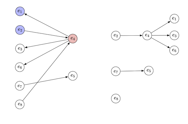
The border graph of our example is depicted in Figure 3 (a).
If a node $e_i \in L$ has no incoming arcs, it means adding $e_i$ to $I$ doesn’t create a circuit in $M_1$, that is, $I + e_i \in \cal I_1$. This property makes them appropriate roots for searching for augmenting paths, so we’ll call each of them a source. Conversely, if a node $e_i \in L$ has no outgoing arcs, it means adding $e_i$ to $I$ doesn’t create a circuit in $M_2$ and we call it a sink.
Let’s interpret what traversing a directed path in this graph means. We start from a source node $e_1$ (a generic node, not the one from the example), which corresponds to adding it to $I$. If it’s also a sink, it doesn’t form a circuit in $M_2$, so $I + e_1$ is feasible. Otherwise we can follow any of the outgoing arc to a node $e_2$ on the right side, which corresponds to removing it from $I + e_1$. This is a feasible solution but no better than what we had, so we need to follow an arc back to the left side.
This will lead us to a node $e_3$ on the left side. The arc $(e_2, e_3)$ says $e_3$ forms a cycle in $M_1$ but $e_2$ breaks it. Since we’re already assuming $e_2$ is being removed from $I$, adding $e_3$ to $I + e_1 - e_2$ is feasible for $M_1$. If $e_3$ is a sink, it’s feasible for $M_2$ as well. Otherwise we keep going.
We define a directed path that starts at a source and ends at a sink as a source-sink path. We might be inclined to think any source-sink path is an augmenting sequence but this is not quite true. However, if we add the condition that a source-sink path from source $e_1$ to $e_t$ is the shortest possible, then the equivalence holds.
Another way to say a source-sink path is the shortest is that it doesn’t admit a shortcut, i.e. if the source-sink path is $e_1, e_2, \cdots, e_t$, then there’s no arc $(e_j, e_k)$ such that $k - j \ge 2$. This is what Theorem 3 states:
Theorem 3. If a source-sink path in $BG(I)$ admits no shortcut, then it forms an augmenting sequence for $I$.
Thus if we use breadth-first search (BFS) starting from the nodes with in-degree 0, we’re invariably looking for shortest paths. A possible BFS on our example is shown in Figure 3 (b).
Thanks to this result, at any point in the BFS we can look for augmenting sequences without explicit knowledge of which edges we have visited so far, that is, we only need knowledge about the initial $I$, but we don’t have to keep computing $I \oplus S_i$ during the search.
Matroid Intersection Algorithm
The ideas from above allows us to come up with an algorithm to solve the matroid intersection problem. We start with an empty set $I$ which is a feasible solution.
We then perform a BFS in the border graph $BG(I)$ in search of augmenting sequences. If we find one, we can stop immediately and augment the set $I$ to obtain a larger feasible solution $I’$.
We repeat the process with $I’$ until we can’t find any augmenting sequence via BFS in which case we can claim we have an optimal solution.
Python Implementation
Matroids are interesting from the implementation point of view in that they provide an abstraction over graphs and other data structures, so this is a good opportunity to leverage object oriented programming.
My first design was to define an abstract class Matroid and have a PartitionMatroid inherit from it. Turns out the algorithm mostly relies on the independent set, even though this independent set encodes the “properties” of specific a matroid as we’ll see soon. To that end, we define a class IndependentSet:
from typing import Generic, TypeVar

TElement = TypeVar('TElement')
class IndependentSet(Generic[TElement]):
    """
    Models an independent set of a matroid M(A, I).
    We assume TElement is hashable.
    """
    pass
We use mypy (i.e. type annotations) to improve readability. An IndependentSet is basically an enhanced Set so we start by defining set-specific APIs:
from abc import ABC, abstractmethod
...
class IndependentSet(Generic[TElement]):

    @abstractmethod
    def add(self, element: TElement) -> None:

    @abstractmethod
    def remove(self, element: TElement) -> None:

    @abstractmethod
    def get_elements(self) -> Set[TElement]:

    @abstractmethod
    def __len__(self) -> int:

    @abstractmethod
    def __contains__(self, element: TElement) -> bool:
We use @abstractmethod to make sure derived classes will implement the logic. In addition to these methods, we also define get_circuit():
from abc import ABC, abstractmethod
...
class IndependentSet(Generic[TElement]):
    ...
    @abstractmethod
    def get_circuit(self, element: TElement) -> Optional[Set[TElement]]:
        """
        Determine if adding e forms a circuit in this matroid.
        If not, return None. Otherwise return a set with elements
        from the circuit.
        """
As we’ve seen in the theoretical section, circuits will be used to define the edges to the graph. We’re now ready to define the independent set for the partition matroids.
Let’s now go to the algorithm. The top level is simple: we keep trying to find augmenting sequences until we can’t, at which point we have an optimal solution.
def intersect(
    elements: TElement,
    s1: IndependentSet[TElement],
    s2: IndependentSet[TElement]
):
    while True:
        seq = find_augmenting_seq(elements, s1, s2)
        if seq is None:
            return s1
        update_solution(s1, s2, seq)
Whenever we find a augmenting sequence we call update_solution() which leverages the .add() and .remove() API from IndependentSet.
The only detail worth commenting is that we perform all the deletions first so s1 and s2 are always valid independent sets. This is important because then implementation of classes deriving from IndependentSet can rely on this assumption as we’ll show.
def update_solution(
    s1: IndependentSet[TElement],
    s2: IndependentSet[TElement],
    seq: List[TElement]
):
    for i in range(1, len(seq), 2):
        s1.remove(seq[i])
        s2.remove(seq[i])
    for i in range(0, len(seq), 2):
        s1.add(seq[i])
        s2.add(seq[i])
The top level implementation of find_augmenting_seq() consists in building the edges of border graph based on the .get_circuit() and initilizing the queue from the BFS with the sources. Then it visits the front of the queue until we finds a augmenting path:
def find_augmenting_seq(
    elements: List[TElement],
    s1: IndependentSet[TElement],
    s2: IndependentSet[TElement],
):

    parents: Dict[TElement, TElement] = {}
    visited: Set[TElement] = set()
    candidates: Queue = Queue()
    left_adj: Dict[TElement, Set[TElement]] = {}
    right_adj: Dict[TElement, Set[TElement]] = {}

    # ...
    # auxiliary functions:
    #
    # def visit_neighbors()
    # def get_sequence()
    # def visit_element()
    # ...

    for e in elements:
        if e in s1:
            continue

        circuit = s1.get_circuit(e)
        # e can be added to s1
        if circuit:
            candidates.put(e)
        else: # can't be added
            for re in circuit:
                if re not in left_adj:
                    left_adj[re] = set()
                left_adj[re].add(e)

        circuit = s2.get_circuit(e)
        if circuit:
            right_adj[e] = circuit

    while not candidates.empty():
        u = candidates.get()
        found_solution = visit_element(u)
        if found_solution:
            return get_sequence(u)
We opted to implement the auxiliary functions as nested functions so we can use the variables like parents, visited, candidates, left_adj and right_adj without passing them as parameters or defining an artificial class.
The function visit_element() is straightforward:
def visit_element(u):
    visited.add(u)

    if u in s1: # right partition
        if u in left_adj:
            visit_neighbors(u, left_adj[u])

    else: # left partition
        if u in right_adj:
            visit_neighbors(u, right_adj[u])
        else: # found solution!
            return True

    return False
The function visit_neighbors() is also simple:
def visit_neighbors(u, neighbors):
    for v in neighbors:
        if v not in visited:
            candidates.put(v)
            parents[v] = u
We just need to remember to save the parent so we can backtrack to retrieve the elements in the augmenting sequence, done by get_sequence():
def get_sequence(u):
    seq = []
    while u is not None:
        seq.append(u)
        u = parents.get(u, None)
    return seq
And that’s it! We worked at a general matroid level, but let’s attempt to solve a concrete problem using special types of matroids.
Bipartite Matching
We can compute the bipartite matching via the intersection of two matroids, partition matroids [5] in particular. Let $G(L, R, E)$ be a bipartite graph with a left partition $L$ and right partition $R$ and set of edges $E$.
We can have a matroid $M_1(E, \cal I_1)$ where the set of edges $I$ is in $\cal I_1$ iff no two edges in it are incident to a vertex in $L$, and $M_2(E, \cal I_2)$ where $I \in \cal I_2$ iff no two edges in it are incident to a vertex in $R$. If we take their intersection $I \in \cal I_1 \cap \cal I_2$ iff no two edges in it are incident to either $L$ or $R$, in other words it represents a bipartite matching!
If we use the matroid intersection algorithm for these matroids we’ll find the maximum cardinality bipartite matching. We’ll assume an edge is a tuple of (int, int) where the first entry represent a vertex on the left partition and the second on the right partition.
The independent sets for the left and right partitions are very similar, differing only on which vertex from an edge it uses to calculating circuits. We thus will define a class BipartiteIndependentSet which takes the side argument indicating which partition it refers to.
TEdge = Tuple[int, int]
class BipartiteIndependentSet(IndependentSet[TEdge]):
    def __init__(self, side: Side):
        self._incidence: Dict[int, TEdge] = {}
        self._side = side
The self._incidence[v] map stores the edge incident to vertex v on the corresponding partition. Since the constraint is that independent set cannot have more than one edge incident to a given vertex, we can store a single edge. This is leveraging the guarantee the intersect() never leave an independent set in an invalid state, a fact we mentioned before.
The implementation of the IndependentSet interface is quite simple. The only detail worth commenting on is the auxiliary get_vertex() which behaves differently for left and right partitions:
class BipartiteIndependentSet(IndependentSet[TEdge]):
    ...
    def get_vertex(self, edge: TEdge):
        (l, r) = edge
        return l if self._side == Side.LEFT else r

    def add(self, edge: TEdge) -> None:
        v = self.get_vertex(edge)
        assert v not in self._incidence
        self._incidence[v] = edge

    def get_circuit(self, edge: TEdge) -> Optional[Set[TEdge]]:
        v = self.get_vertex(edge)
        if v in self._incidence:
            return set([self._incidence[v], edge])
        return None

    def get_elements(self) -> Set[TEdge]:
        return set(self._incidence.values())

    def remove(self, edge: TEdge) -> None:
        v = self.get_vertex(edge)
        del self._incidence[v]

    def __len__(self) -> int:
        return len(self._incidence)

    def __contains__(self, edge: TEdge) -> bool:
        v = self.get_vertex(edge)
        return v in self._incidence and edge == self._incidence[v]
With that in place, we can use intersect() to implement a maximum cardinality bipartite matching:
def bipartite_matching(edges):
    left = BipartiteIndependentSet(side=Side.LEFT)
    right = BipartiteIndependentSet(side=Side.RIGHT)
    result = intersect(edges, left, right)
    return result.get_elements()
The code for the bipartite matching using matroid intersection is available on Github.
Complexity
The rank of a matroid represents the size of the largest independent it contains, so the largest feasible solution is bounded by the minimum of the ranks between $M_1$ and $M_2$. In other words, if $R_1$ is the rank of the matroid $M_1$ and $R_2$ of the matroid $M_2$, the size of the optimal solution is bounded by $R = \min(R_1, R_2)$.
Thus the loop in intersect() executes at most $R$ times, since it has to improve the solution on every iteration. The function find_augmenting_seq() performs a BFS so it’s bounded by the number of edges in the border graph. So if $m = \abs{A}$, the border graph could have partitions of size $O(m)$ and be complete, so in the worst case it could have $O(m^2)$ edges.
In addition find_augmenting_seq() also has to build the graph. For each of the $m$ elements, we call get_circuit(). We can assume the cost of finding a circuit is $O(c)$.
In [2] Lawler uses a more specific bound: let $b$ be the cost of determining whether a given set belongs to $\cal I$ (i.e. is independent). Then the cost of finding a circuit is $O(Rb)$. To see why, consider this algorithm for obtaining a circuit from $I + e$: try to remove one element at a time from $I$, checking at every step if the resulting set is independent. Suppose when we remove element $e’$ we reduce it to $I’$ and that $I’ + e$ is independent. In the step before removing $e’$ we had a circuit (i.e. minimal dependent set). Since $\abs{I}$ is $O(R)$, the complexity of this is $O(Rb)$.
Thus the overall complexity of the algorithm is $O(Rm^2 + R^2mb)$ or $O(Rm^2 + Rmc)$.
For the bipartite matching case, $m$ is the number of edges in the original graph and $R$ is $O(n)$, where $n$ is the number of vertices. The cost of finding a circuit is $O(1)$ since we’re using a lookup hash table and the circuit size is always 2, which gives us a $O(nm^2)$, less efficient than Ford–Fulkerson algorithm’s $O(nm)$.
Conclusion
I’ve first heard of matroid intersection back during undergrad but never got to learn it. After over about 15 years I finally managed to do it!
The idea is relatively intuitive, trying to greedly improve the solution on one side and then greedly fix on the other side, but the reason why it works is less obvious.
I’m still not done with matroids though. I want to learn about weighted matroid intersection before moving on.
Appendix
In this appendix we provide proofs to the theorems used in the post.
Theorem 1. If $I \in \cal I$ and $I + e \not \in \cal I$, then $I + e$ constains exactly one circuit.
Proof. Let’s prove by contradiction and assume there are distinct circuits $C_1$ and $C_2$ in $I + e$. First recall that by the first property of matroids, any subset of an independent set is also an independent set (hypothesis $H_{1.1}$). Next recall that a circuit is a minimum dependent set, so removing any edge from it turns it into a independent (hypothesis $H_{1.2}$).
Since $C_1$ and $C_2$ are different, we can find $e’ \in C_1 \setminus C_2$ (hypothesis $H_{1.3}$). Since $C_1$ is a circuit $C_1 - e’ \in \cal I$ (by $H_{1.2}$). Also, since $C_1 - e \subseteq I$ and $C_2 - e \subseteq I$ (both by $H_{1.2}$), then $(C_1 \cup C_2) - e$ is independent. This means that by applying the second property of matroids multiple times, it’s possible to augment $C_1 - e’$ with elements from $(C_1 \cup C_2) - e$ to obtain $I’$ such that $\abs{I’} = \abs{(C_1 \cup C_2) - e}$.
Since we only used elements from $C_1$ or $C_2$ to augment $C_1 - e’$, $I’ \subseteq C_1 \cup C_2$. Given that $\abs{I’} = \abs{(C_1 \cup C_2) - e} = \abs{C_1 \cup C_2} - 1$, this means there exist exactly one element $e’’ \in (C_1 \cup C_2) \setminus I’$. First, suppose that while augmenting $C_1 - e’$ we didn’t add $e’$ into $I’$. Since $e’ \in C_1 \subseteq C_1 \cup C_2$ (by $H_{1.3}$), then it must be that $e’’ = e’$ and since $e’ \not \in C_2$, this implies that the only element missing from $I’$ comes exclusively from $C_1$, so it contains all elements from $C_2$ and thus $C_2$ is an independent set (by $H_{1.1}$), which is a contradition.
Conversely, assume we added $e’$ into $I’$ while augmenting $C_1 - e’$. Then $I’$ contains $C_1$, which means $C_1$ is an independent set (by $H_{1.1}$), which is also a contradition. QED.
Theorem 2. If no augmenting sequence exists for $I$, then $I$ is of maximum cardinality.
Proof. Let’s prove the contrapositive, i.e. that if $I$ is non-optimal (Hypothesis $H_{2.1}$), then there is an augmenting sequence. From $H_{2.1}$, there is $J$ such $\abs{J} \gt \abs{I}$. Given the first property of matroids if $J \in \cal I$, any of its subsets is also in $\cal I$ which means we can find a subset $J$ with a cardinality exactly one larger than $I$’s, i.e. $\abs{J} = \abs{I} + 1$.
This let’s us use Lemma 3.1 to show a source-sink path $S$ exists in $BG(I)$. For any source-sink path it’s possible to remove its shortcuts by simply taking them, so we can assume a shortcut-free source-sink path exists in $BG(I)$ and thus Theorem 4 applies, and we have an augmenting sequence. QED.
Lemma 2.1 Let $I, J$ be intersections such that $\abs{J} = \abs{I} + 1$. There exists a source-sink path $S$ in $BG(I)$ such that $S \subseteq I \oplus J$.
Proof sketch. Consider the subgraph $H$ of $BG(I)$ induced by the vertex set $J \oplus I$. The left partition will have the nodes $J \setminus I$ and the right the nodes $I \setminus J$. First we handle the case where there are isolated vertices on the left, meaning they’re both sources and sinks and that we can add any of them to $I$ to obtain a larger feasible solution and we’re done.
Assume otherwise that none of the sources and sinks are isolated. We split the arcs of $H$ into those that go from right to left, $A_1$, and those from left to right, $A_2$. It’s possible to show there’s a subset of $A_1$ (ignoring the direction for now) that is a matching $X_1$ covering all nodes on the left side except those that are sources. Similarly, there’s a subset of $A_2$ (again, ignoring the direction) that is a matching $X_2$ covering all nodes on the left side except those that are sinks.
If we take the subgraph $H’$ of $BG(I)$ induced by the arcs $X_1 \cup X_2$, we have that:
- Sources have exactly one outgoing arc (that from $X_2$),
- Sinks have exactly one incoming arc (that from $X_1$),
- Other nodes have exactly one outgoing and one incoming arc (one from each of $X_1$ and $X_2$).
In other words, $H’$ consists of disjoint components that are either directed paths or cycles. Since the paths start on a source and end on a sink they must be augmenting paths. Now we have that the left side of $H’$ has more nodes than the right side, because $\abs{J \setminus I} \gt \abs{I \setminus J}$.
Since cycles have the same number of nodes from each side, the difference in size must be made up by a path, so there must exist at least one augmenting path. QED.
Theorem 3. If a source-sink path in $BG(I)$ admits no shortcut, then it forms an augmenting sequence for $I$.
Proof. Let $S = (e_1, \cdots, e_t)$ a source-sink path in $BG(I)$. Since the source and sink nodes are both on the left partition this path has to have an odd length. We’ll first show this path corresponds to an alternating sequence by showing it satisfies properties (1) to (3). Property (1) is trivially satisfied since by definition $e_1$ is a source node and thus can be added to $M_1$, so $I + e_1 \in \cal I_1$.
For property (2) we’ll prove that for all even $i$ and $S_i = (e_1, \cdots, e_i)$, $I \oplus S_i \in \cal I_2$. We define $I^{(k)} = I + e_k - e_{k+1} \cdots + e_{i - 1} - e_i $ for odd $1 \le k \le i - 1$. Suppose by inductive hypothesis that $I^{(k)} \in \cal I_2$. Our induction is done backwards so our base is $k = i - 1$. We have that $I^{(i - 1)} = I + e_{i - 1} - e_i$ which must belong to $\cal I_2$ because that’s the condition for $(e_{i-1}, e_j)$ to exist.
We claim that $I^{(k)} + e_{k-2}$ has a circuit. Suppose this is not true. We know that $I + e_{k-2}$ has the circuit $C_{e_{k-2}}^{(2)}$ because of the arc $(e_{k-2}, e_{k-1})$. Since $I^{(k)}$ is $I$ with some elements added and other removed, for $I^{(k)} + e_{k-2}$ to not contain $C_{e_{k-2}}^{(2)}$, one of the removed elements, say $e_j$ for $j$ odd and $j \ge k$ must be in $C_{k-2}^{(2)}$, to “break” that circuit. This however would imply the existence of arc $(e_{k-2}, e_j)$ which would represent a shortcut for our path which contradicts our assumption that our path is shortcut-free. Thus we conclude that $I^{(k)} + e_{k-2}$ not only has a circuit but it’s $C_{k-2}^{(2)}$.
We have that $I^{(k)} \in \cal I_2$, $I^{(k-2)} = I^{(k)} + e_{k - 2} + e_{k - 1}$ and that $e_{k-1} \in C_{k-2}^{(2)}$, given the arc $(e_{k-2}, e_{k-1})$. We know then that removing arc $e_{k-1}$ breaks the circuit created by adding $e_{k - 2}$ to $I^{(k)}$ so $I^{(k-2)}$ continues to be independent in $M_2$. Thus if we use $k = 1$ we have $I \oplus S_i \in \cal I_2$.
Analogous reasoning can be done to show it a source-sink path in $BG(I)$ satisfies condition (3). So the source-sink path in $BG(I)$ is an alternating path with odd length, so it remains to show $I \oplus S \in \cal I_2$ for it to be an augmenting one.
We can use induction. We’ll prove that $(I \oplus S_i) + e_t \in \cal I_2$, for even $i$. Our base case is $i = 2$ so we must show $I + e_1 - e_2 + e_t \in \cal I_2$. Since $e_t$ is a sink, $I + e_t \in \cal I_2$ and by construction $I + e_1 - e_2 \in \cal I_2$. Since $\abs{I + e_t} = \abs{I + e_1 - e_2} + 1$, we can use the second property of matroids to show that there exists $e \in (I + e_t) \setminus (I + e_1 - e_2)$ such that $I + e_1 - e_2 + e \in \cal I_2$. The only possibilities are $e_t$ or $e_2$, but adding $e_2$ to $I + e_1 - e_2$ leaves us with $I + e_1$ which is not in $\cal I_2$, since arc $(e_1, e_2)$ exists. Thus it must be $e_t$ that gives us $I + e_1 - e_2 + e_t \in \cal I_2$.
Now given the inductve hypothesis that $(I \oplus S_k) + e_t \in \cal I_2$ for $k$ even, we need to show it holds for $k + 2$ as well. Again, since $(I \oplus S_k) + e_t$ and $I \oplus S_{k+2}$ are independent sets, and $\abs{(I \oplus S_k) + e_t} = \abs{I \oplus S_{k+2}} + 1$ there must exist $e \in (I \oplus S_k + e_t) \setminus (I \oplus S_{k+2})$ such that $I \oplus S_{k+2} + e \in \cal I_2$. The only candidates are $e_t$ and $e_{k+2}$. Adding $e_{k+2}$ to $I \oplus S_{k+2}$ gives us $I \oplus S_{k+1}$ which is not in $\cal I_2$, since arc $(e_{k+1}, e_{k+2})$ exists. It must then be $e_t$ that gives us $(I \oplus S_{k+2}) + e_t \in \cal I_2$.
By setting $i = t-1$, we arrive at $I \oplus S \in \cal I_2$, showing at last that the path $S$ is an augmenting sequence. QED.
Related Posts
The Hungarian Algorithm. We’ve mentioned this in the post but there are parallels between bipartite matching and matroid intersections. In the bipartite matching the “unit” is an edge, while in a matroid $M(A, \cal I)$ is a element in $A$. A matching is analogous to a feasible solution $I \in \cal I_1 \cap \cal I_2$ and an augmenting path is an augmenting sequence.
Recap
- What is a circuit? Circuits are minimal dependent sets.
- Recall that a border graph $BG(I)$ is a directed bipartite graph. What is on left and right partitions? How are the arcs defined? The right partition are elements in $I$ while the left partition are the rest. A left-to-right arc $(l, r)$ means that $I + l$ contains a circuit $C^{(2)}$ in $M_2$ and $r \in C^{(2)}$. A right-to-left arc $(r, l)$ means $I + l$ contains a circuit $C^{(1)}$ in $M_1$ and $r \in C^{(1)}$.
- What are sources and sinks in $BG(I)$? Sources are vertices on the left partition with no incoming arc, sinks are vertices on the right partition with no outgoing arc.
- How to find an augmenting sequence in $BG(I)$? BFS starting at any source until finding a sink.
