kuniga.me > NP-Incompleteness > The Hungarian Algorithm

The Hungarian Algorithm

02 Dec 2022

Harold William Kuhn was an American mathematician, known for the Karush–Kuhn–Tucker conditions and the Hungarian method for the assignment problem [1].

According to Wikipedia [2], Kuhn named the algorithm Hungarian method because it was largely based on the earlier works of Hungarian mathematicians Dénes Kőnig and Jenő Egerváry.

However in 2006, the mathematician Francois Ollivier found out that Carl Jacobi (known for Jacobian matrices) had already developed a similar algorithm in the 19th century in the context of systems of differential equations and emailed Kuhn about it [6].

One fascinating coincidence is that Jacobi is Kuhn’s ancestral advisor according to the Mathematics Genealogy Project! [5]. Here’s the ancestry chain (year when they got their PhD in parenthesis):

• Harold William Kuhn (1950)
• Ralph Hartzler Fox (1939)
• Solomon Lefschetz (1911)
• William Edward Story (1875)
• Carl Gottfried Neumann (1856)
• Friedrich Julius Richelot (1831)
• Carl Gustav Jacob Jacobi (1825)

If this genealogy is to be trusted, I wonder if Kuhn was aware of this fact, given he wrote about Jacobi’s life in [6].

In this post we’ll explore this algorithm and provide an implementation in Python.

The Balanced Assignment Problem

Suppose we have a bipartite graph with a set of vertices $S$ and $T$ of same size $n$, with a set of edges $E$ edges between them associated with a non-negative weight. A matching $M$ is a subset of $E$ such that no two edges in $M$ are incident to the same vertex. A perfect matching is one that covers every vertex. The weight of a matching is the sum of weighs of its edges.

The balanced assignment problem asks to find the perfect matching with the maximum weight. We can reduce several variants of this problem to this specific version.

Negative weights

We can assume all the weights are non-negative. If there are negative weights, let $W$ be the smallest weight. We add $W$ to all edges so they’re now non-negative. Since the perfect matching has exactly $n$ edges, we just need to discount $nW$ from our solution.

Incomplete graph

We can assume the bipartite graph is complete. If the original graph is not, we can always add artificial edges with weight 0 and remove them later from the solution without affecting the optimal value.

If it’s incomplete and has negative weights, we can simply ignore those by setting those to 0. A matching of maximum weight does not include any negative edges unless we also require the matching to be of maximum cardinality. In this case the reduction to the problem at hand is non-trival.

Unbalanced assignment

We can assume that both partitions have the same size. If in the original graph they aren’t, we can add artificial vertices (and then make them complete as above) and remove edges incident to them later from the solution without affecting the optimal value.

Integer Linear Programming

We can formulate the assignment problem as follows. Suppose we’re given weights $w_{ij}$ for $1 \le i, j \le n$. We introduce binary variables $x_{ij}$ where $x_{ij} = 1$ indicates the edge $(i,j)$ is in the matching.

The objective function is thus:

Subject to:

Let’s find the dual of this ILP. Constraints (1) map to variables we’ll name $u$ and constraints (2) map to variables we’ll name $v$.

Subject to:

It’s possible to show that if there are feasible solutions $x^{*}_{ij}$ and $u^{*}_i$, $v^{*}_j$ such that their objective functions are equal, that is,

then they’re optimal solutions for their respective formulations. Another characterization of optimizality is that the variables satisfy the complementarity constraints:

Another way to have these constraints:

The Hungarian algorithm

The Hungarian algorithm aims to solve the ILP by finding solutions that satisfy (1)-(9). Initially we set

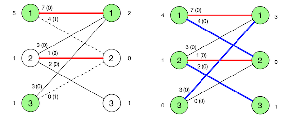
Figure 1 depicts an example from [5] which we’ll use throughout this post. It displays the value of variables such $u$ (to the left of the $S$ partition), $v$ (to the right of the $T$ partition), $w_{ij}$ (along the corresponding edge) and the difference $u_i + v_j - w_{ij}$ (defined as slack later, in parenthesis).

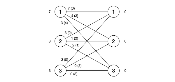
We can verify this satisfies all constraints except (8). The algorithm will then iterate on satisfying these constraints without ever violating the other ones. We’ll now describe a high-level way to do this.

Max matching in induced graph

First, consider the graph $G(u,v)$ which is the original bipartite graph but only with those edges $(i, j)$ satisfying $u_i + v_j = w_{ij}$. We call such edges tight, whereas those with $u_i + v_j \gt w_{ij}$ are loose. The amount to remove from $u_i + v_j$ of a loose edge to turn it into a tight edge is called slack and denoted by $\delta = u_i + v_j - w_{ij}$.

From our initial choice of $u$ every node in $S$ has at least one tight edge incident to it. To see why, let $j_i$ such that $w_{ij_i} = \max(w_{ij}) = u_i$. Since $v_{j_i} = 0$, we have $u_i + v_{j_i} = w_{ij_i} + 0 = w_{ij_i}$. Thus edge $(i,j_i)$ is in $G(u,v)$.

We then try to find a maximum cardinality matching $M_{uv}$ in $G(u,v)$. If we find a perfect match (i.e. cardinality $n$), then setting $x_{ij} = 1$ for edges in the matching will satisfy (8) and we’re done.

If not, we need to add edges to $G(u,v)$ by manipulating $u$ and $v$ such that the resulting $G(u,v)$ will allow a bigger matching. We need some theory first.

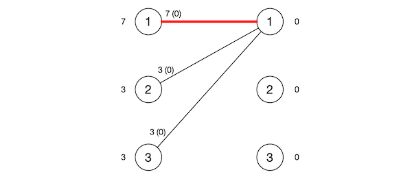
Figure 2 shows the induced graph corresponding to our initial example where the edges are tight and the red bold edge is some maximal matching in such graph.

Berge’s theorem

We note that the matching $M_{uv}$ is also a matching in the original graph. Since the original graph is complete it has to have a perfect match, so $M_{uv}$ is not maximal there. We’ll now see how to increase or augment the size of $M_{uv}$.

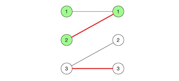
Let $M$ be a matching in a bipartite graph. We define an alternating path in $M$ as a path in the graph whose edges alternate between those in the matching and those not. If no edge in the matching is incident to a vertex $v$, we say the vertex is unmatched. If an alternating path starts and ends in an unmatched vertex, we call it an augmenting path.

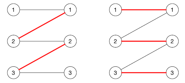
The reason it’s called augmenting is that it’s can be used to increase the size of a matching. The augmenting path necessarily has an odd number of edges, say $2k + 1$, and $k + 1$ of these edges are not in the matching, while $k$ are. We can increase the matching by 1 by simply putting all edges not in the matching into the matching and vice-versa. Figure 3 has an example.

Berge’s theorem states that a matching $M$ in a graph is maximum if and only if there is no augmenting path in $M$. This implies that if the matching is not maximal, there must exist an augmenting path we can use to increase the size of $M$.

Starting from the fact that $M_{uv}$ is maximal in $G(u,v)$ but not in $G$, we can use Berge’s theorem to claim there is an augmenting path $P$ in $G$ that doesn’t exist in $G(u,v)$.

How can we find $P$? We first need to introduce an auxiliary structure.

Forest of alternating paths

Let $r$ be an unmatched vertex from $S$. Traverse the graph from $r$ but only following alternating edges and do not visit any vertex more than once. One way to achieve this is to orient the edges: for every edge in $(i,j) \in G(u,v)$ with $i \in S, j \in T$, we orient $i \rightarrow j$ if $(i,j)$ is not in $M_{uv}$ and orient $j \rightarrow i$ otherwise. Then we can just do a BFS in this directed graph from $r$. Let $C(r)$ be the tree corresponding to such traversal.

Repeat this for every other unmatched vertex in $S$, with the care not to visit any vertex that belongs to some other tree. The result of these traversals is a collection of disjoint trees, or forest of alternating paths which we’ll call $F$.

Note that this forest does not necessarily contain all edges from the matching.

Adding edges to the forest

We can manipulate $u$ and $v$ in order to add an edge to $F$. Consider some edge $(x, y)$ where $x \in S$ and $x \in F$, $y \in T$ and $y \not \in F$ and defined as a frontier edge. Let $\delta = u_x + v_y - w_{xy}$. If we subtract $\delta$ for all $u_i$, $i \in F \cap S$ and add $\delta$ for all $v_j$, $j \in F \cap T$, it’s easy to see that all edges in $F$ will continue to be tight. Since we didn’t add $\delta$ to $v_y$ but subtracted from $u_x$, edge $(x, y)$ is now tight.

However, by doing this we might violate (4), i.e. $u_i + v_j \ge w_{ij}$, for some edges. Suppose there is another frontier edge $(x’, y’)$ with slack $\delta’ = u_x’ + v_y’ - w_{x’y’} \lt \delta$. We have that $u_x’ + v_y’ - \delta’ = w_{x’y’}$. If we subtract $\delta$ from $u_x’$ and leave $v_y’$ unchanged, we get $u_x’ + v_y’ - \delta \lt u_x’ + v_y’ - \delta’ = w_{x’y’}$ which violates (4).

To avoid this, we choose the smallest slack $\delta$ among all frontier edges. We’re guaranteed to add at least one edge to the forest $F$ without violating any new constraints. Figure 6. shows an example.

Now with $(x, y)$ added, we have that either $y$ is unmatched which means we just found an augmenting path, or $y$ is part of an edge $(x’, y)$ in the matching that is not reachable by any of the root vertices in $F$, but we can now add it to $F$, since $(x, y) + (x’, y)$ is alternating.

Once we find an augmenting path $P$ and “flip” the edges to increase the matching $M_{uv}$ by one, we need to recalculate the forest of alternating paths because the first vertex of $P$ is no longer unmatched.

Every time we do a change of dual variables we either increase the matching size by one, or increase the forest by 2 edges. When we increase the matching, we recalculate the forest so we can’t assume the size of the tree will remain constant, but even if tree was emptied out every time that happened, there would still be a ceiling of $O(n^2)$ change of dual variables that can happen.

This proves the algorithm finishes. Let’s now prove it is correct.

Optimality

Suppose by contradition that there are no frontier edges in $F$ and the corresponding matching $M_{uv}$ is not perfect. By Berge’s theorem, there is an augmenting path $P$ for $M_{uv}$ in $G$.

Let $r$ be its first vertex. By definition, it’s unmatched and w.l.o.g. assume it’s in $S$ and thus root of some tree in $F$. Let $(i, j)$ be the first edge that doesn’t belong to $C(r)$. There are a few scenarios to consider.

Case 1. Suppose $(i, j)$ exists in $G(u,v)$. This is possible because we might not add an edge $(i,j)$ to $C(r)$ if the vertex $j$ has already been visited by some other tree, rooted at $r’$. This is the same as Case 2.2.

Case 2. Suppose $(i, j)$ does not exist in $G(u,v)$. We have that $i$ belongs to $F$ (because we’re assume the edge $(i, j’)$ preceding $(i, j) \in P$ exists in $F$). We have now 2 subcases:

Case 2.1 $j \not \in F$. Then $(i, j)$ is a frontier edge but that contradicts our initial hypothesis. Hence this case can’t happen.

Case 2.2 $j \in F$. Then $j$ belongs to the tree of another root $r’$. Let $Q$ be the (alternating) path from $r’$ to $j$ and $P_j$ be the part of path $P$ starting at $j$ and $P_i$ the part of path $P$ ending in vertex $i$. Since $P_i$ belongs to the tree of $r$, it’s disjoint of $Q$ and hence $Q + P_j$ forms a path, it’s an augmenting one and it has at least one fewer edge not in $F$ than $P$, so this eventually reduces to Case 2.1.

Python Implementation

With the ideas discussed above we are ready to implement this algorithm. There are three major routines: building the alternating path forest, augmenting an augmenting path and changing the dual variables.

Let’s start with augment():

def augment(self, j):
  while j is not None:
    i = self.parent[T][j]
    self.match[T][j] = i
    self.match[S][i] = j
    j = self.parent[S][i]

In this method parent[.][x] is the parent of vertex x in the forest. match[.][x] is the index of the vertex matched with x. T is an alias to 1 and S to 0. I’ve opted to use a $2 \times n$ matrix to store information about the vertices on the bipartite graph.

The idea is simple: we start an unmatched $j \in T$ so we know that the edge $(i, j)$ with its parent $i$ is not in the match, so we can match $i$ and $j$. Note that $i$ was matched with its parent $j’$, but we don’t need to unmatch because $j’$ will be eventually rematched.

Next we explore change_duals():

def change_duals(self):
  delta = min(v for v in self.slack if v > 0)

  for i in range(self.n):
    if self.visited[S][i]:
      self.u[i] -= delta

  for j in range(self.n):
    if self.visited[T][j]:
      self.v[j] += delta
    # frontier edge
    elif self.slack[j] > 0:
      self.slack[j] -= delta
      # note: self.parent[j] has been set
      # during the forest visit
      if self.slack[j] == 0:
        self.candidates.put((1, j))

Here slack[j] represents the slack for $j \in T$. If slack is positive then (parent[T][j], j) is either a frontier edge or it’s an unreacheable vertex, in which case slack[j] = INF so delta = min(...) works.

Then we proceed to subtract delta from u and add to v. We also update slack to keep it consistent with u and v. visited[.][x] indicates whether the vertex belongs to the forest.

We finally have an optimization: if slack[j] became 0, we added j to the forest, so we can continue building the forest from j instead of doing it from scratch.

We now define visit_forest():

def visit_forest(self):
  while not self.candidates.empty():
    [side, c] = self.candidates.get()

    if self.visited[side][c]:
      continue
    self.visited[side][c] = True

    if side == S: # c in S
      self.visit_s(c)
    else: # c in T
      augmented = self.visit_t(c)
      if augmented:
        return True

  return False

This method basically implements a BFS using a queue. The current nodes to be visited are stored in candidates. We have to handle vertices in $S$ and $T$ differently.

When visiting $T$, there’s a chance we find an augmenting path. If we do, we’ll need to restart the construction of the forest, so we have to short-circuit.

For $i \in S$ we call visit_s():

def visit_s(self, i):
  # update pi from edges not in match
  for j in range(self.n):
    if self.match[S][i] == j:
      continue

    slack = self.u[i] + self.v[j] - self.adj[S][i][j]
    if slack < self.slack[j]:
      self.slack[j] = slack
      self.parent[T][j] = i

      # edge (i,j) is now in the forest. keep visiting
      if slack == 0:
        self.candidates.put((1, j))

We first observe that we skip visiting its match. That’s because if $(i, j) \in M_{uv}$, then we arrived at $i$ from $j$ already.

We just need to update the slacks from its neighbors in $T$ in $G$. Note that we update the slack and parent even for edges that are not in $G(u, v)$. This is important for the change_duals(), since once we change u and v the slack on that edge might go to 0 and cause it to be added.

For $j \in T$ we call visit_t():

def visit_t(self, j):
  i = self.match[T][j]
  # found an augmenting path
  if i is None:
    self.augment(j)
    return True

  self.parent[S][i] = j
  self.candidates.put((0, i))
  return False

If $j$ is unmatched, we found an augmenting path so we can call augment(j) and stop trying to visit/construct the forest.

Otherwise we keep constructing the alternating trees by following the edge from the match (recalling that j was reached from a non-match edge).

We can put it together in expand_matching():

def expand_matching(self):
  self.init_candidates()
  self.init_parent()
  self.init_visited()
  self.init_slack()

  while True:
    augmented = self.visit_forest()
    if augmented:
      return

    self.change_duals()

We first reset all the variables so we can the recreate the forest from scratch. The only non-trivial init_* function is init_candidates() which initializes the candidates queue with all the unmatched vertices from $S$.

Then we do a mix of BFS exploration with dual variable changes until we are able to augment an augmenting path. Finally the main routine solve():

def solve(self):
  self.init_match()
  self.init_u()
  self.init_v()

  # for each iteration we should increase the matching side
  for t in range(self.n):
    self.expand_matching()

  return sum(self.u) + sum(self.v)

First we initialize the dual variables and the match which don’t need to be reset during the execution of the algorithm. Recalling that init_u() starts with the maximum weight of edges incident to each vertex in $S$:

def init_u(self):
  u = [0]*self.n
  for i in range(self.n):
    for j in range(self.n):
      u[i] = max(u[i], self.adj[S][i][j])

  self.u = u

It then calls the expand_matching() function n times. Each expand_matching() increases the matching size by at least one, so this is enough to find the optimal matching.

After the loop, since u and v are optimal, we can use the objective function of the dual ILP which is a bit simpler to compute than adding the weights of the edges in the matching.

The full Python implementation as well as a C++ implementation one are available on Github.

Runtime complexity

We argue that expand_matching() is $O(n^2)$, the cost of doing a BFS on the graph. Even when we call change_duals() we don’t re-do the BFS from scratch but continue from where we stopped, so we visit each edge at most once in expand_matching().

We only reset the BFS once we do augment() but we only do it $O(n)$ times through the algorithm, so the total runtime complexity is $O(n^3)$.

Conclusion

I was studying the Hungarian method from Lawler’s Combinatorial Optimization: Networks and Matroids [3] and it was incredibly hard to convert the provided pseudo-code into a working implementation.

I missed several details like the fact that the graph has to be complete and the partitions of the same size (without these conditions, the algorithm is unable to find augmenting paths correctly) . There’s vagueness about in which order to visit vertices and terminology.

What ultimately helped me understand the algorithm in detail was Topcoder’s article [4] and Wikipedia [2].

The Hungarian is another one of the algorithms I used multiple times but never understood in detail until writing about it, like the KMP.

Related Posts

An Introduction to Matroids - In that post we talk about the greedy algorithm for finding minimum/maximum spanning tree, known as the Kruskal algorithm. The idea behind the change of dual variables in the Hungarian algorithm vaguely reminds me of the Kruskal algorithm, in which we choose the edge with lowest weight to add to the existing forest.

Lagrangian Relaxation - Duality is utilized in Lagrangian Relaxation to obtain upper bounds (in case of maximization) for branch-and-bound algorithms.

Totally Unimodular Matrices - The incidence matrix of a bipartite graph is totally unimodular (TU). This allows deriving the König-Egerváry theorem (the Hungarians) which says that maximum cardinality matching and minimum vertex cover are duals in bipartite graphs.

As we described, the Hungarian algorithm uses maximum cardinality matching as a sub-routine. There’s a variant which we didn’t mention which uses minimum vertex cover as sub-routine [2] (see Matrix interpretation).

References

• [1] Wikipedia: Harold W. Kuhn
• [2] Wikipedia: Hungarian Algorithm
• [3] Combinatorial Optimization: Networks and Matroids, Eugene Lawler.
• [4] Topcoder: Assignment Problem and Hungarian Algorithm
• [5] Mathematics Genealogy Project
• [6] A tale of three eras: The discovery and rediscovery of the Hungarian Method, Harold W. Kuhn.

Source code | RSS feed | Tags: combinatorial optimization, graph theory, integer programming