kuniga.me > NP-Incompleteness > Single Digit Speech Recognition via LPC + DTW
Single Digit Speech Recognition via LPC + DTW
25 Mar 2022
In this post we’ll attempt the speech recognition of single digits using deterministic algorithms, in particular Linear Predictive Coding (LPC) [1] and Dynamic Time Warping (DTW) [2].
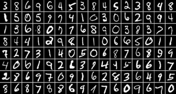
Digit recognition is one of the first problems we try to solve when learning image recognition so I found reasonable to try the same with speech recognition.
We’ll provide implementation in Python and the results of simple experiments.
Experiment Setup
Data
I recorded myself pronouncing digits from 0 to 9 a few times. I used one of the sets as the test data and the rest as training data. They are stored in the test and train variables respectively.
We’ll be transforming the data in several ways, so we define a transform_data() utility which accounts for the different structure of train and test data:
def transform_data(train, test, tr):
    dig_cnt = len(test)
    tr_train = [0]*len(train)
    for t in range(len(train)):
        tr_train[t] = [None]*dig_cnt
        for i in range(dig_cnt):
            tr_train[t][i] = tr(train[t][i])

    tr_test = [0]*dig_cnt
    for i in range(dig_cnt):
        tr_test[i] = tr(test[i])

    return (tr_train, tr_test)
Running the Experiment
For each digit in the test set, we compare with the training digits and measure the average distance for each pair of digits. The overall experiment runner looks like this:
def experiment(training_data, test_data, cost_f):
    dig_cnt = len(test_data)
    test_cnt = len(training_data)
    results = np.empty(shape=(dig_cnt, dig_cnt))

    for i in range(dig_cnt):
        for j in range(dig_cnt):
            d = 0
            for t in range(test_cnt):
                d += cost_f(training_data[t][i], test_data[j])
            results[i][j] = d / test_cnt
    return results
Display
We define a make_table() that creates a styled Pandas dataframe. Each row corresponds to the digits in the test set and the columns to the digits on the training set. The cell value is the average distance between the data (smaller is better). We highlight the actual best match (i.e. for each row the column with minimum value). If it’s the expected one (in the diagonal), we color it green otherwise red.
See any of the experiment results for an example.
Experiment 1: Dynamic Time Warping
The first experiment we tried was comparing the input signals without any pre-processing using FastDTW (a fast approximated version of DTW). We wrote our own version of it in [1], but we use the fastdtw Python package since it’s more battle-tested.
from fastdtw import fastdtw

def fastdtw_cost(s1, s2):
    return fastdtw(s1, s2)[0]

make_table(experiment(train, test, fastdtw_cost))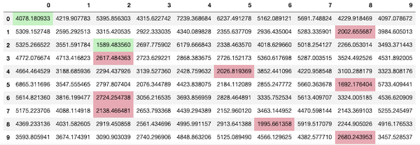
As we can see from Figure 2 it’s not very effective. My main suspicion is that there’s a lot of silence in the recordings and they might be adding to the DTW distance. It’s also not efficient: it took 18 minutes to run!
Experiment 2: Trimming Silence
I tried a few methods to trim silence at the beginning and end of the recording. The one that fared best was to first remove noise from the signal and then ignore samples from the beginning and end until the moving average (to avoid outliers) of the amplitude first surpass a threshold.
To remove noise I used the Python package noisereduce. The overall trimming process is as follows:
import noisereduce
def trim_silence(samples):
    samples = noisereduce.reduce_noise(y=samples, sr=sample_rate)
    marks = detect_silence(samples)
    return samples[marks[0]: marks[1]]
To determine the indices to trim, we search for the first time the moving average surpasses 2% of the maximum amplitude:
def detect_silence(samples):
wlen = int(sample_rate / 1000 * window_ms)
max_amp = np.max(samples)
abs_samples = np.abs(samples)
threshold = 0.02 * max_amp
wsum = np.sum(abs_samples[0:wlen])
li = 0
while li + wlen < len(abs_samples) and wsum / wlen <= threshold:
wsum += abs_samples[li + wlen] - abs_samples[li]
li += 1
wsum = np.sum(abs_samples[-wlen:])
ri = len(abs_samples) - 1 - wlen
while ri > 0 and wsum / wlen <= threshold:
wsum += abs_samples[ri] - abs_samples[ri + wlen]
ri -= 1
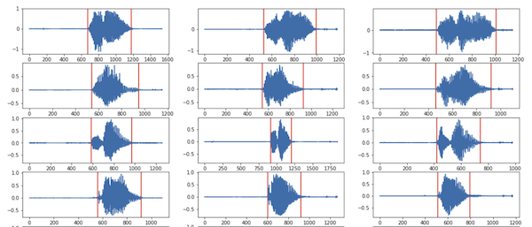
return [li, ri + wlen]We can visualize the result by adding vertical markers where we detected the start/end of silence. Figure 3 shows it works relatively well, accounting for the fact I had to fine tune the threshold to achieve this.
In this experiment we compare the input signals after the silence removal, still using fastdtw().
(trimmed_train, trimmed_test) = transform_data(train, test, trim_silence)
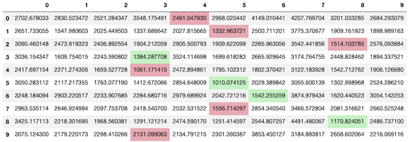
make_table(experiment(trimmed_train, trimmed_test, fastdtw_cost))Figure 4 shows that the results are slightly better and a bit faster (6 min) but far from useful.
Silence Detection in Frequency Domain
One other method to detect silence I tried and I think it’s worth mentioning is doing the analysis in the frequency domain.
We assume that during silent periods we only have white noise, which is spectrally flat. In other words if we analyze the frequencies of a small window corresponding to a silence, we’d expect them to be evenly distributed.
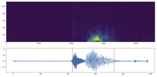
A good way to visualize this is via a spectrogram, which is essentially a heatmap where the x-axis is time and y-axis the frequency. We divide the signal into overlapping blocks and compute the FFT at each block and plot the amplitude of the frequencies. See the top of Figure 5 for an example.
To detect silence we compute the variance of the frequencies for each block and assume it’s silence if it’s a fraction of the maximum variance. See the bottom of Figure 5 for an example.
This method seems to work better than looking for small amplitudes in time domain if there’s noise. However I found that once we apply noisereduce.reduce_noise() the version in time domain seemed to do better overall.
Experiment 3: Applying LPC
In addition to trimming the silence, we can encode the signal using LPC. The idea is that the encoded signal better captures the “essence” of the signal and makes it less susceptible to noise and distortions.
For each signal we’ll chunk it into overlapping blocks (with length corresponding to 30ms) and encode each block using 6 poles as in [2] and discard the white noise generator (G below). We use lpc_encode() function as defined in [2].
def get_lpc_coeff(samples):
    sym = False # periodic
    w = hann(floor(0.03*sample_rate), sym)
    p = 6 # number of poles
    [A, G] = lpc_encode(samples, p, w)
    return A
Each block will have 6 values corresponding to each of the poles. If we take all the blocks over time we have 6 series. We can visualize the LPC coefficients in a heatmap (y-axis representing poles, x-axis the blocks) for a few digits (row) and sets (column):
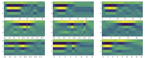
We can see from Figure 6 that the heatmaps in each row have similar overall color pattern, which is a good indication. We can turn the multiple series into one multi-valued series, so it can be fed into fastdtw(). This is done via convert_series():
# Turns multi-series into single series w/ multi y-value
def convert_series(series_set):
    series_cnt = len(series_set)
    series_len = len(series_set[0])
    single_series = []
    for t in range(series_len):
        ys = np.empty(shape=series_cnt)
        for i in range(series_cnt):
            ys[i] = series_set[i][t]
        single_series.append(ys)
    return single_series

def get_as_lpc(samples):
    return convert_series(get_lpc_coeff(samples))
Then we run fastdtw() over the transformed data. Fortunately fastdtw() supports multi-valued y-axis out of the box.
(lpc_coeff_train, lpc_coeff_test) =
  transform_data(trimmed_train, trimmed_test, get_as_lpc)

make_table(experiment(lpc_coeff_train, lpc_coeff_test, fastdtw_cost))
Figure 7 shows that the results look much better! All but one digit was mis-categorized.
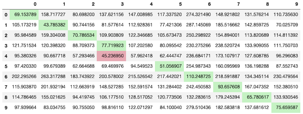
It also ran pretty fast, 0.8s! I think we might be able to improve the results by adding more training data, given that we only used 2 sets for training and one for testing.
Here is the list of parameters I had to tweak. Unfortunately the quality of the results is quite sensitive to them.
| Parameter | Values Tried (*: best) |
|---|---|
| Window overlap | 0.4*, 0.5, 0.6 |
| Window size | 10ms, 30ms* |
| Number of poles | 3, 6*, 12 |
| Silence Threshold | 0.01, 0.02*, 0.05 |
All the code including the code to plot the charts (but excluding the data) are available as a Jupyter notebook.
Conclusion
In this post we attempted single digit speech recognition. We experimented with using FastDTW directly on the original signal, FastDTW on the signal without silence and FastDTW on the LPC coefficients.
Only the FastDTW+LPC combo yielded reasonable results. I used just a couple of samples but also only attempted recognizing my own speech, which is a much easier problem to solve than general recognition. For my ultimate goal this is not an issue though.
Before doing this experimentation I was assuming we just needed LPC to make the code run faster but it turns out it also improves accuracy, which is counter-intuitive given LPC is a lossy process and takes much less space. This suggests that DTW is not the best way to compare speech directly.
The idea of using DTW+LPC came from Rabiner’s paper [3], which claims that for single word recognition this method outperforms stochastic methods like Hidden Markov Models.
My next challenge is to perform detection in real time. We can still pre-process the training data but have to match the test one as it comes.
