kuniga.me > NP-Incompleteness > Dynamic Time Warping
Dynamic Time Warping
25 Jan 2022
Suppose we are given two discrete signals corresponding to the speech resulting from pronouncing a given sentence. They might have been pronounced by different people and in different intonations and speed, and we would like determine the similarity between these signals.
In this post we’ll discuss dynamic time warping, a technique that can be used to compare the similarity between time series allowing for small variances in the time scales. We’ll provide Python implementations of an exact algorithm $O(N^2)$ based on dynamic programming and an approximated one that runs in $O(N)$.

Euclidean Matching
One simple way to solve this problem is by normalizing/interpolating both the amplitudes and the time frame and see compute the difference between each timestamp.
For example, suppose we’re given the time series [1, 3, 3, 2] and [10, 18, 27, 30, 28, 25, 20]. We could normalize the amplitudes of the second time series as [1, 1.5, 2.7, 3, 2.8, 2.5, 2] (i.e. divide by 10) and then interpolate the first one so the number of elements is the same [1, 1.5, 3, 3, 3, 2.5, 2], then assume a 1:1 matching. This is called the Euclidean matching.
This assumes some linear scaling between the two series with a factor that is constant across the time range which might not be true. We want a more dynamic way to match points in these series to account for this. Figure 1 shows the problem with Euclidean matching by showing what the actual matching is.
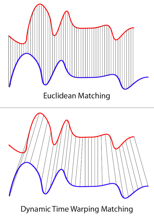
Note that the “distance” between consecutive matches is not constant, so normalizing by a single constant factor would not help.
Dynamic Programming
Let $\vec{x}$ and $\vec{y}$ be signals represented by arrays of floats (uniform sampling) with lengths $n$ and $m$, respectively.
We can map multiple points from $\vec{x}$ to a single one in $\vec{y}$ and vice-versa, based on how close in amplitude points are. For example, suppose x = [1, 1, 3, 5, 2] and y = [1, 3, 6, 3, 1]. We can use the following match:
x      | y
[1, 1] | [1]
[3]    | [3]
[5]    | [6]
[2]    | [3, 1]
We’ll call a match a pair of points, one from each series that we think correspond to each other. Note that a point from one series might belong to multiple matches with points from other series. A list of all match pairs is called a path.
We define the distance between two time series as the sum of distances between each pair in a path, so for the example above:
x      | y      | d
[1, 1] | [1]    | 0 + 0
[3]    | [3]    | 0
[5]    | [6]    | 1
[2]    | [3, 1] | 1 + 1
The total distance is 3. A different match could be mapping [5] to [6,3]:
x      | y      | d
[1, 1] | [1]    | 0 + 0
[3]    | [3]    | 0
[5]    | [6, 3] | 1 + 2
[2]    | [1]    | 1
with a total distance of 4. The constraint of our matching are:
Constraint 1: Every element from both $\vec{x}$ and $\vec{y}$ must belong to at least one match.
Constraint 2: The matches cannot “cross”. That is, if we match $x_i$ with $y_j$, then for any $i’ \ge i$ and a match of $x_{i’}$ with $y_{j’}$ it must be $j’ \ge j$.
We can then define an optimization problem: given those constraints, minimize the total distance of the match.
This can be solved by dynamic programming. Let $D_{i,j}$ be the minimum matching distance for the sequences $x_0, \cdots x_{i-1}$ and $y_0, \cdots y_{j-1}$. Suppose we already know the solution for $D_{i-1,j-1}$, $D_{i,j-1}$ and $D_{i-1,j}$.
There are few cases to consider:
Case 1: $x_{i-1}$ and $y_{j-1}$ will form a new matching pair, adding a distance of $\abs{x_{i-1} - y_{j-1}}$ to the total, and we can then extend the solution from $D_{i-1,j-1}$.
Case 2: $y_{j-1}$ is already paired up with one or more elements in $\vec{x}$, and we’ll add $x_{i-1}$ to the match, which also adds $\abs{x_{i-1} - y_{j-1}}$ to the total, and we can extend from $D_{i-1,j}$.
There’s a hypothetical case here to point out: it could be the case that both $y_{j-2}$ and $y_{j-1}$ are already matched to $x_{i - 2}$ and by pairing $y_{j-1}$ with $x_{i - 1}$ would create a “zig-zag” match ($y_{j-2} \rightarrow x_{i - 2} \rightarrow y_{j-1} \rightarrow x_{i-1}$), which is undesirable. In this case though, we could “un-match” $y_{j-1}$ and $x_{i - 2}$, which would discount $\abs{x_{i-2} - y_{j-1}}$ from the total distance and then we could have chosen Case 1 with a cost that is no greater than Case 2.
So as long as we break ties by picking Case 1 first we’ll avoid this case.
Case 3: is the analogous to Case 2 but switching $x_{i - 1}$ for $y_{j-1}$, and we can extend from $D_{i,j-1}$.
This gives us a simple recurrence for computing $D_{i,j}$:
\[D_{i,j} = \min (D_{i-1,j-1}, D_{i,j-1}, D_{i-1,j}) + \abs{x_{i-1} - y_{j-1}}\]It remains to define the base case, $D_{0,0}$, which is matching empty vectors, for a distance of 0. The Python code is then relatively straightforward:
def dtw(xs, ys):
    n, m = len(xs), len(ys)

    opt = np.full((n+1, m+1), np.inf)
    opt[0, 0] = 0

    for i in range(1, n+1):
        for j in range(1, m+1):
            opt[i, j] = abs(xs[i-1] - ys[j-1]) + \
                min([opt[i-1, j], opt[i, j-1], opt[i-1, j-1]])

    return opt[n][m]
The running time of the algorithm is clearly $O(nm)$ and uses $O(nm)$ space as well.
Reconstructing the Matching
We can obtain the path by backtracking on the memoization matrix. We need to modify dtw() to return the matrix instead of the optimal solution value.
def dtw(xs, ys):
    # ...
    return opt

def dtw_path(xs, ys):
    opt = dtw(xs, ys)

    i = len(opt) - 1
    j = len(opt[-1]) - 1

    # note that opt's range are shifted by 1, so we
    # need to subtract 1 to obtain xs's and ys's
    # indexes
    path = [[i - 1, j - 1]]
    while i > 0:
        if (opt[i - 1, j - 1] < opt[i - 1, j] and
            opt[i - 1, j - 1] < opt[i, j - 1]):
            i, j = i - 1, j - 1
        elif opt[i - 1, j] < opt[i, j - 1]:
            i = i - 1
        else:
            j = j - 1

        if i > 0 and j > 0:
            path.append([i - 1, j - 1])

    # reverse backtrack order
    return path[::-1]
Computing the cost of the solution given the path is easy:
def compute_cost_from_path(xs, ys, path):
    cost = 0
    for [i, j] in path:
        cost += abs(xs[i] - ys[j])
    return cost
Windowing
The rationale behind windowing is that it’s very unlikely that points from the beginning of one time series will end up being matched with the ones at the end of the other. They’re likely to be around the same neighborhood, or window.
Let $w$ be the length of the window. Then we only need to look at $O(w)$ points for each $i$, for example $(i - w, i + w)$, leading to a $O(nw)$ complexity. If $w$ is constant or at least much smaller than $m$ it can speed things up.
We can also reduce the space usage to $O(nw)$ by considering each row of the opt matrix to be a moving window. It makes working with indices really tricky, but if we don’t reduce space usage, just initializing the matrix will incur in a $O(nw)$ runtime complexity. We’ll provide an implementation of the windowed DTW later.
The biggest hurdle with the static window approach is determining the right size for the window, which might depend a lot on the data, for example if the signals are shifted by some significant amount on rare occasions.
Can It Be Faster?
According to Wikipedia [2], Gold and Sharir came up with a $O(n^2 / \log \log (n))$ algorithm (which I’d bet is much slower than the $O(n^2)$ in practice).
However according to [2], Bringmann and Künnemann proved that no strongly subquadratic algorithm exists unless P=NP, which means that a much more efficient algorithm such as $O(n \log n)$ is unlikely to exist.
There are several heuristic algorithms which give good approximate results and run fast in practice. Let’s take a look at one of them, FastDTW.
FastDTW
As we discussed, using a fixed window around $i$, i.e. $(i - w, i + w)$, could be problematic. This assumes that the matching $j$ in $\vec{y}$ lies within that window, or requires us to make the window too big, leading to an inefficient algorithm.
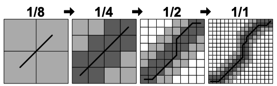
The idea of FastDTW is to use dynamic window sizes that are not necessarily centered in $i$. To compute this window it first solves the problem at a smaller resolution. More specifically, if the initial $\vec{x}$ and $\vec{y}$ had sizes $n$ and $m$, it constructs $\vec{\overline{x}}$ and $\vec{\overline y}$ with half of their sizes $\lfloor \frac{n}{2} \rfloor$ and $\lfloor \frac{m}{2} \rfloor$ by averaging every 2 adjacent points.
Once we have a path, i.e. a list of pairs of $i, j$ found for $\vec{\overline x}$ and $\vec{\overline y}$, the assumption is that the path for $\vec{x}$ and $\vec{y}$ will follow the same overall trajectory, thus it can inform where to search for matches between $\vec{x}$ and $\vec{y}$.
For instance, say that index $i$ is matched with $j$, $j+1$ and $j + 2$ in the reduced problem. Then in the original problem we can assume the indexes $2i$ and $2i + 1$ will be matched within $2j$ to $2(j + 2) + 1$, so we can use that as a window! To be safe, we can also add a constant margin of safety.
We claims that the amortized window size is constant. To see why, note that the length of the window for a given $i$ is proportional to the size of its matching plus a constant, but the sum of all matching sizes is $O(n + m)$, so is the total window sizes. This means that if we solve the windowed DTW using these windows, in total we’ll only be looking at $O(n + m)$ elements.
We keep solving halved versions of the problem recursively until the problem gets small enough that it can be solved by a regular DTW. Figure 3 depicts this idea.
Complexity
Suppose for simplicity that the sizes of $\vec{x}$ and $\vec{y}$ are both equal $N$. At a given step of the recursion, we can compute $\vec{\overline x}$ and $\vec{\overline y}$ which can be done in $O(N)$, and can compute the windowed DTW in $O(N)$. The recursive step will take $O(N/2)$, so adding all steps will lead to $N + N/2 + N/4 + \cdots = O(N)$.
The size of the problem for the base case is a constant, so overall the algorithm runs in $O(N)$.
Let’s now implement these ideas.
Implementation
Windowed DTW. First let’s generalize the dtw() implementation to take an optional window range, which determines the ranges of $j$’s to look for for each $i$.
def get_absolute_j(i, j, wrange):
    if wrange is None:
        return j
    return min(wrange[i][0] + j, wrange[i][1])

def get_relative_j(i, j, wrange):
    if wrange is None:
        return j
    return max(j - wrange[i][0], 0)

def get_neighbors(i, abs_j, opt, wrange):
    neighbors = []
    for [di, dj] in [[-1, -1], [-1, 0], [0, -1]]:
        i2 = i + di
        j2 = get_relative_j(i2, abs_j, wrange) + dj
        if j2 >= 0 and j2 < len(opt[i2]):
            neighbors.append([i2, j2])
    return neighbors

def windowed_dtw(xs, ys, wrange = None):

    n, m = len(xs), len(ys)

    if wrange is not None:
        assert len(wrange) == n + 1

    opt = []
    for i in range(n + 1):
        jmin, jmax = wrange[i] if wrange else [0, m - 1]
        opt.append(np.full(jmax - jmin + 1, np.inf))

    for i in range(1, n + 1):
        for j in range(len(opt[i])):

            abs_j = get_absolute_j(i, j, wrange)

            # special case: value = 0 for empty series
            if i == 1 and abs_j == 0:
                opt[i][j] = abs(xs[i - 1] - ys[abs_j])
            else:
                neighbors = get_neighbors(i, abs_j, opt, wrange)

                min_value = min(
                    [opt[i2][j2] for [i2, j2] in neighbors]
                )

                opt[i][j] = min_value + abs(xs[i - 1] - ys[abs_j])

    return opt
Implementation notes:
(1) There’s some tricky index business here. The “actual” $j$ from one row doesn’t map directly to other row’s $j$, since the windows have different offsets, so we need to normalize. We use get_absolute_j() and get_relative_j() to convert between these domains.
(2) We need check for boundaries. In the simple dtw() all was handled by virtual of having the same range and using sentinels. We use get_neighbors() to abstract these checks and only return adjacent cells that fit the window sizes.
(3) We don’t have a sentinel for j=0 anymore, so we have to handle the base opt[0][0] as a special case.
Matching from windowed ‘matrix’. Recovering the path from opt is similar to dtw_path but remembering that opt is not a full matrix.
def path_from_windowed_opt(opt, wrange = None):
    i = len(opt) - 1
    # j is relative to the windowed row
    j = len(opt[-1]) - 1

    path = []

    while i > 0:

        abs_j = get_absolute_j(i, j, wrange)
        path.append([i - 1, abs_j])

        neighbors = get_neighbors(i, abs_j, opt, wrange)

        min_value = min([opt[i2][j2] for [i2, j2] in neighbors])

        # set i,j to the first neighbor that yields the optimal solution
        [i, j] = next(
            [i2, j2] for [i2, j2] in neighbors \
                if opt[i2][j2] == min_value
        )

    # reverse backtrack order
    return path[::-1]
Getting window from low-res path. Once we know the path at half of the resolution, we can use it do define the window range for each $i$.
def get_search_window(path, n, m, radius):

    # initialize with empty ranges
    wrange = [None]*(n + 1)
    wrange[0] = [0, m - 1]

    def add_range(i, jmin, jmax):
        w = wrange[i]
        if w is not None:
            jmin = min(w[0], jmin)
            jmax = max(w[1], jmax)
        wrange[i] = [clamp(jmin, 0, m-1), clamp(jmax, 0, m-1)]

    for i, j in path:
        imin, imax = 2*i, 2*i + 1

        jmin, jmax = 2*j - radius, 2*j + 1 + radius
        add_range(imin, jmin, jmax)

        if imax < n:
            add_range(imax, jmin, jmax)

    # fill in ranges that were not set with defaults
    for i in range(len(wrange)):
        if wrange[i] is None:
            wrange[i] = [0, m - 1]

    return wrange
Note that the same i may appear multiple times in path, so we need to update the existing range.
Lowering resolution. Getting the low-res version of a series is the easiest part, we just need to make sure to handle sequences with odd length!
def halve(xs):
    new_xs = []
    n2 = len(xs)//2
    for i in range(n2):
        new_xs.append((xs[2*i] + xs[2*i+1])/2)

    # odd number of points
    if len(xs) % 2 == 1:
        new_xs.append(xs[-1])

    return new_xs
With these helper functions we can now define the body of fast_dtw():
def fast_dtw(xs, ys, radius = 30):
    min_size = radius + 2
    if len(xs) <= min_size or len(ys) <= min_size:
        opt = windowed_dtw(xs, ys)
        return path_from_windowed_opt(opt)

    lowres_xs = halve(xs)
    lowres_ys = halve(ys)

    lowres_path = fast_dtw(lowres_xs, lowres_ys, radius)

    wrange = get_search_window(lowres_path, len(xs), len(ys), radius)

    opt = windowed_dtw(xs, ys, wrange)
    return path_from_windowed_opt(opt, wrange)
Experiments
Data
To test the results we used the speeches provided in [1] and trimmed them to a much smaller size since we also want to run the $O(nm)$ algorithm with it. The speeches we use are:
- (A) Doors and Corners, Kid. That’s where they get you. [v1]
- (B) Doors and Corners, Kid. That’s where they get you. [v2]
Derived data:
sample_a_1k- a segment of (A) of size ~1,000sample_a_10k- a segment of (A) of size ~10,000sample_b_1k- a segment of (B) of size ~1,000sample_b_10k- a segment of (B) of size ~10,000samples_c_1k- a segment of (A) of size ~1,000 in a different part of the speech
Performance
We ran dtw(), fast_dtw() (radius of 30) and windowed_dtw() (fixed window size of 100) with (sample_a_1k, sample_b_1k). We also ran fast_dtw() and windowed_dtw() with (sample_a_10k, sample_b_10k). The results are summarized in the table below:
| Function | n = 1,000 | n = 10,000 |
|---|---|---|
dtw() |
3.9719s |
- |
fast_dtw() |
0.5138s |
4.3631s |
windowed_dtw() |
0.7693s |
3.4498s |
We can see that fast_dtw() and windowed_dtw() are much faster than dtw() for $N = 1000$, and that it grows linearly: when we use a 10x bigger input, it takes about 10x the time.
Accuracy
Here we compare the difference in the values of the solutions returned by dtw() (ground truth), fast_dtw() (radius of 30) and windowed_dtw() (fixed window size of 100), for series (sample_a_1k, sample_b_1k) and (sample_a_10k, sample_b_10k).
| Function | n = 1,000 | n = 10,00 |
|---|---|---|
dtw() |
263,733 |
- |
fast_dtw() |
264,161 (0.16%) |
17,506,397 |
windowed_dtw() |
278,763 (5.70%) |
21,571,474 |
In terms of accuracy fast_dtw() does much better than windowed_dtw(). The latter could do especially bad if the series are similar but are very shifted in relation to each other.
Differentiation
One important property of distance metrics is that it is small for things that are similar and big for things that are not.
We compare the costs of between the similar (sample_a_1k, sample_b_1k) and different (sample_a_1k, samples_c_1k) series.
| Series | Distance |
|---|---|
sample_a_1k, sample_b_1k |
263,733 |
sample_a_1k, samples_c_1k |
2,933,360 |
We can see that distance between (sample_a_1k, sample_b_1k) is much smaller than between (sample_a_1k, samples_c_1k). Note that the absolute distance doesn’t tell us about similarity on itself, but can be used for comparison.
The cost depends on the length of the series and the magnitude of their amplitudes, so we might need to do some normalization on the series to make sure we’re comparing series with similar length and range of amplitude.
Source Code
The implementation and experiments are available on Github as a Jupyter notebook. I haven’t included the actual data but it can be obtained from [1].
Post Image
The image on the top of post was created by plotting sample_a_1k and sample_b_1k and drawing a line between points of each based on their optimal matching. We used matplotlib and the code is available on Github with the rest of the code. I found it looked pretty nice!
Conclusion
To recap, in this post we learned about the dynamic time warping problem and how it can be solved via dynamic programming in $O(N^2)$, which might not be fast enough for practical applications. Further, it’s unlikely an exact algorithm exists that much faster than that.
Thus, there are many approximated alternatives with results that are both fast and accurate in practice, one being FastDTW. The idea behind it is very clever: it solves a low-res version of the problem and uses the solution to guide the search for the full-res one.
I struggled a lot with the implementation of FastDTW, especially trying to map indices between absolute and relative domains. The initial version of my code was really complex, so I spent quite some time cleaning it up. One particular abstraction that simplified things is get_neighbors(): it hides the complexity of checking boundaries for each of the 3 neighbors.
The recurrence for DTW reminds me of the one for computing the edit distance between words. I didn’t know it had a name, but according to Wikipedia it’s called Wagner–Fischer algorithm.
