kuniga.me > NP-Incompleteness > Pitch Detection via Cepstrum in Python

Pitch Detection via Cepstrum in Python

11 Dec 2021

In this post we’ll implement a pitch detector using cepstrum. In our Cepstrum post, we covered the basic theory and showed why cepstrum can be useful to determine the pitch of human speech.

Cepstrum Theory Recap

Let $\vec{x}$ be an input signal and $\mathscr{F}(\vec{x}, \omega)$ is the DTFT of $\vec{x}$ and $\mathscr{F}^{-1}(\vec{x})$ the inverse DTFT. The real Cepstrum is defined as:

\[\hat x_t = \mathscr{F}^{-1}(\ln \abs{\mathscr{F}(\vec{x}, \omega)})\]

Separating Source and Filter

In Cepstrum we reviewed that the signal for human speech, represented by $\vec{x}$, is a convolution of a excitation source $\vec{e}$ (vocal chords) and a impulse response $\vec{h}$ from the filter (vocal tract):

\[\vec{x} = \vec{e} * \vec{h}\]

We’ve also seen that the contribution of $\vec{h}$ to the cepstrum tends to be concentrated in the small values of quefrencies, so if we can try to filter small values to recover the fundamental frequency of $\vec{e}$, also know as the pitch.

We know that the pitch for human voice is typically between 85Hz and 255Hz [4], so we only need to look at entries in the cepstrum corresponding to that range.

Scipy’s FFT

Scipy provides an implementation of the (Cooley-Tukey) FFT algorithm [1]. The expression ys = fft(xs) implements the following equations:

\[y_k = \sum_{t = 0}^{n-1} e^{-2 \pi i \frac{kt}{n}} x_t, \qquad k = 0, \cdots, n-1\]

and its inverse xs = ifft(ys) implements:

\[x_t = \frac{1}{N} \sum_{k = 0}^{n-1} e^{2 \pi i \frac{kt}{n}} y_k \qquad t = 0, \cdots, n-1\]

Note the output of fft() has the same size as the input xs. For k = 0, we can see ys[0] is just the sum of the elements in xs.

Assume n = len(xs) is even. Then the first half ys[1:n/2 - 1] contains positive frequencies while the second half ys[n/2:n-1] contains the negative frequencies in decreasing order. That is, if we were to sort ys by frequency, it would look like: [ys[n-1], ys[n-2], ..., y[n/2], y[0], y[1], ..., y[n/2 - 1]]. A similar distribution applies for n odd.

Scales

The fft() is unitless in the sense it doesn’t need to know about the sample rate of the input signal. The scale of the output does depend on it though.

More specifically, let r be the sample rate (in Hertz) and n the number of samples in the input signal. The total period covered by xs is n/r (in seconds). The granularity of the frequencies represented by ys is r/n (in Hertz).

So for example, if the sample rate is 8kHz and we provide 10 samples to the fft(), the response will have a granularity of 800, so correspond to the frequencies:

[0, 800, 1600, 2400, 3200, -4000, -3200, -2400, -1600,  -800]

This is exactly what fftfreq(n, 1/r) calculates for us.

Cepstrum in Python

Thus the cepstrum can be defined as a one-liner using Numpy and Scipy:

import numpy as np
from scipy.fft import fft, ifft

def compute_cepstrum(xs):
    cepstrum = np.abs(ifft(np.log(np.absolute(fft(xs)))))

Pitch Detection

Windowing

Because the pitch can vary across a long speech, we’ll break it down in small chunks with assumption that within that time window the pitch is constant. Like we did in the Linear Predictive Coding (LPC), we can use the Overlap-Add Method (OLA) to create overlapping windows:

# 30ms Hann window
sym = False # periodic
w = hann(floor(0.03*sample_rate), sym)

def create_overlapping_blocks(x, w, R = 0.1):
    n = len(x)
    nw = len(w)
    step = floor(nw * (1 - R))
    nb = floor((n - nw) / step) + 1

    B = np.zeros((nb, nw))

    for i in range(nb):
        offset = i * step
        B[i, :] = w * x[offset : nw + offset]

    return B

B = create_overlapping_blocks(x, w)

I honestly don’t know if OLA is the right method or term in this case because we’ll not have to recover (add) the full signal at the end like we did with LPC, but we do need some windowing.

Human Cepstrum

Once we obtain that cepstrum via compute_cepstrum() we can filter the quefrencies to those within the human pitch range. We note that quefrencies is same domain as the original signal (since it’s the result of a inverse Fourier transform in the frequency domain), so we can obtain it as:

quefrencies = np.array(range(len(xs)))/SAMPLE_RATE_HZ

But the interpretation of a quefrency at $t$ seconds corresponds to the period of a cycle in the signal ys (where ys = fft(xs)). Since we only want to analyze periods in ys corresponding to human pitch range (85 to 255Hz), we exclude periods lower than 1/255 and greater than 1/85. To be safe we use a range of (70-270Hz) in the code:

def compute_human_cepstrum(xs):

    cepstrum = compute_cepstrum(xs)
    quefrencies = np.array(range(len(xs)))/SAMPLE_RATE_HZ

    # Filter values that are not within human pitch range

    # highest frequency
    period_lb = 1/270
    # lowest frequency
    period_ub = 1/70

    cepstrum_filtered = []
    quefrencies_filtered = []
    for i, quefrency in enumerate(quefrencies):
        if quefrency < period_lb or quefrency > period_ub:
            continue

        quefrencies_filtered.append(quefrency)
        cepstrum_filtered.append(cepstrum[i])

    return (quefrencies_filtered, cepstrum_filtered)

Finding Peaks

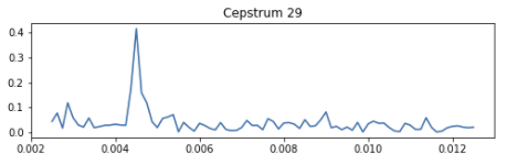
Once we have the filtered cepstrum, we need to detect where the peak is. This can be tricky, especially when there’s no peak, because there’s a lot of confounding noise. Here’s a clear example of a peak:

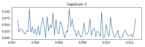
Plot depicting a prominent peak — Figure 1: Clear peak

Here’s an example with a lot of peaks that are mostly noise:

Plot showing several peaks but none is dominating — Figure 2: Noise

The first entry when I Google “detect peak in time series” is this StackOverflow answer [2]. The top answer provides an algorithm that detects deviations from the running moving average to detect peaks.

It takes three parameters:

lag - length of the moving average
threshold - how many standard deviations do we consider a peak to have
influence - the weight between 0 or 1 on how much the current point has on computing the moving average and standard deviations.

I’ve obtained good results with lag = 5, threshold = 10 and influence = 0.5.

If we can’t detect peaks, we return None for the frequency to indicate this is likely noise.

def find_freq_for_peak(quefrencies, cepstrum):

    lag = 5
    threshold = 10
    influence = 0.5
    result = thresholding_algo(cepstrum, lag, threshold, influence)

    # no peaks
    if max(result["signals"]) <= 0:
        return None

    return quefrencies[np.argmax(cepstrum)]

The estimated peak then is the median of the the valid peaks.

Experiments

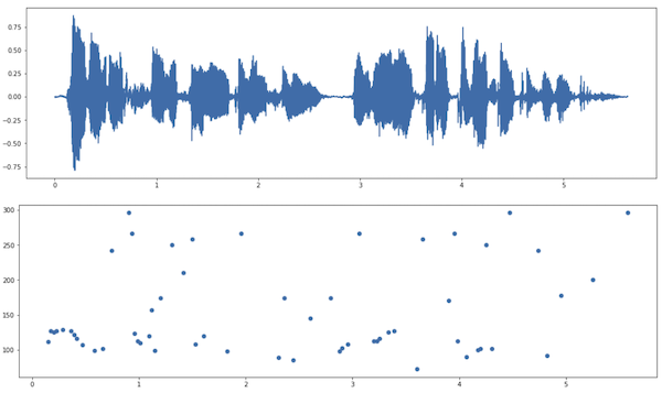
I tried running the pitch detection for a few examples. One is the male voice we used from the Linear Predictive Coding (LPC) post [3], which returns a median of 125Hz which is within the 85 to 155 Hz in [4] for typical male voices.

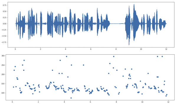
See caption — Figure 3: Male voice results. Top: amplitude of the recording, bottom: scatter plot for the estimated peak for each window.

We can see a clear concentration of pitches around 100-150Hz in the Figure above.

The second example is from a female voice [5] speaking in Catalan. It estimated a pitch of 166Hz which is within the 165 to 255Hz described in [4] for typical female voices.

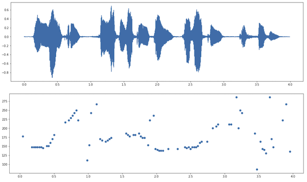
In this example the concentration is not as uniform, with variance over time.

The third example is another male voice [6] also speaking in Catalan. It estimated a pitch of 125Hz.

This one is not as clear cut as the first example and we detected fewer peaks.

The fourth example is my own voice, recorded using my earphone’s microphone in lossless format via QuickTime. It returned an estimate of 242Hz! This is likely inaccurate though, which we can see from looking at the pitch value distribution:

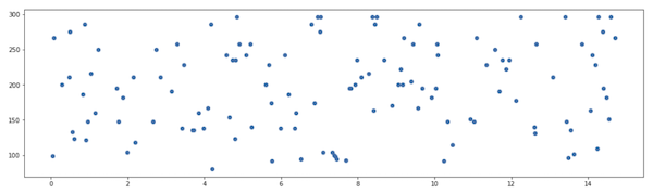
The only explanation I can think of is that I recorded it in a noisy environment which is messing with the results.

Source

The full implementation is on my Github as a Jupyter notebook.

Conclusion

The cepstrum method seems to work fine but is very sensitive to background noise. I didn’t try too many combinations of the parameters, including window size, amount of overlap and the other peak detection parameters. I would also like to investigate methods for removing noise.

As always, having to implement a theory showed I haven’t understood many details, for example the interpretation of the scales of the output of fft() and ifft(), or how to detect peaks.

I found the response format of fft() a bit strange since the entries are not sorted by frequency. I wonder if it’s due to specific implementation details or if it’s a conscious API design, maybe because in most cases people only want the first half of the array? I want to study the implementation of the Cooley-Tukey FFT in the future which might shed some light on this.

Linear Predictive Coding was mentioned in the post. In both we provide Python implementations and use the windowing strategy.

Cepstrum was mentioned in the post as the theory backing this implementation.

Discrete Fourier Transforms discusses 3 types of Fourier Transforms. While in theory we often rely the Discrete-Time Fourier Transform (DTFT), in practice the FFT algorithm solves the Discrete Fourier Series (DTF).

References

[1] Fourier Transforms (scipy.fft)
[2] Peak signal detection in realtime timeseries data
[3] Linear Predictive Coding is All-Pole Resonance Modeling - Hyung-Suk Kim
[4] Voice Frequency
[5] Freesound: speech-female.wav
[6] Freesound: speech-male.wav

| Tags: signal processing python