kuniga.me > NP-Incompleteness > Quantum Phase Estimation
Quantum Phase Estimation
23 Dec 2020
Given a unitary matrix $U$ with eigenvector $\ket{u}$, we want to estimate $\varphi$ where $e^{2 \pi i \varphi}$ is the eigenvalue of $U$.
This serves as framework for solving a varierity of problems including order finding, which as we have shown in a recent post, can be used to efficiently factorize a number.
We assume basic familiarity with quantum computing, covered in a previous post, plus we’ll use quantum Fourier transform (QFT) in one of the steps.
Quantum Circuit
Let’s first consider smaller parts of the circuit before showing the whole picture.
Controlled gate revisited
We described the CNOT gate in [2], and then that any $n$-qubit gate $U$ can be transformed into a $(n+1)$-qubit [3] (the $CR_k$ gate). In both cases the control qubit is assumed to be in the computational basis (more specifically $\ket{0}$ or $\ket{1}$).
Here we consider the case where the control bit is in an arbitrary state, e.g. $\alpha \ket{0} + \beta \ket{1}$.
Suppose we transformed a $n$-qubit gate $U$ into a $(n+1)$-qubit controlled gate. What happens when we apply it to a $(n+1)$-qubit $\ket{c} \ket{y}$ where $y$ is a $n$-qubit and $c$ is the control?
If $c = \ket{0}$, the output is $\ket{y} \ket{0}$ whereas if $c = \ket{1}$ the output is $U \ket{y} \ket{0}$. We can use the linearity principle and obtain
\[(1) \quad \alpha \ket{0} \ket{y} + \beta \ket{1} U \ket{y}\]The $U$ gate
Because $\ket{u}$ is the eigenvector of $U$ and $e^{2 \pi i \varphi}$ its eigenvalue, then by definition $U \ket{u} = e^{2 \pi i \varphi} \ket{u}$, so if we apply a gate with a corresponding unitart matrix $U$ to an input $\ket{u}$ we obtain $e^{2 \pi i \varphi} \ket{u}$.
It’s possible to show that $U^k$ for a positive integer $k$ is also a unitary matrix and thus has a corresponding gate. If we apply it to $U$’s eigenvector $\ket{u}$ we get $e^{2 \pi i k \varphi} \ket{u}$.
A simple circuit
The circuit below is used as a building block for the larger one.
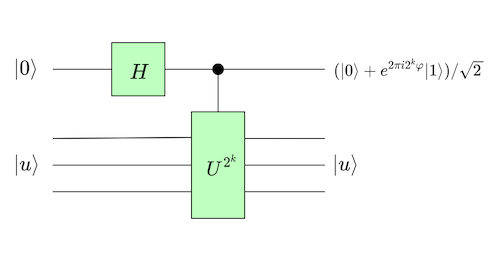
Let’s follow what’s happening. We start with:
\[\ket{\psi_1} = \ket{0} \ket{u}\]In the first step we apply the Hadamard to obtain
\[\ket{\psi_2} = (\frac{\ket{0} + \ket{1}}{\sqrt{2}}) \ket{u}\]Now the first qubit is used as control for the $U^{2^k}$ gate, which similarly to (1) is
\[\frac{\ket{0} \ket{u} + \ket{1} U^{2^k} \ket{u}}{\sqrt{2}}\]Using the fact that $U^{2^k} \ket{u} = e^{2 \pi i 2^k \varphi} \ket{u}$ we have
\[\frac{\ket{0} \ket{u} + \ket{1} e^{2 \pi i 2^k \varphi} \ket{u}}{\sqrt{2}}\]Since $e^{2 \pi i 2^k \varphi}$ is scalar we can do some re-arranging:
\[\ket{\psi_3} = \frac{\ket{0} + e^{2 \pi i 2^k \varphi} \ket{1}}{\sqrt{2}} \ket{u}\]In this view, the first qubit $\ket{0}$ became $\frac{\ket{0} + e^{2 \pi i 2^k \varphi} \ket{1}}{\sqrt{2}}$ while the $n$-qubit $\ket{u}$ remained unchanged, which is a bit counter intuitive especially given the first qubit was the control one.
The whole picture
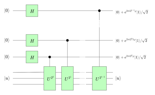
We can see that this circuit combines $t$ of the small circuit from the previous session. The output of $U^{2^i}$ is fed into $U^{2^{i+1}}$ but as we saw above we can assume it doesn’t change the input so the final state would still be $\ket{u}$.
For each of the control qubits, there will be a corresponding $U^{2^k}$, so it will end as $\frac{\ket{0} + e^{2 \pi i 2^k \varphi} \ket{1}}{\sqrt{2}}$ as we saw above.
If we look at the whole state after applying this larger circuit we end up with
\[\frac{ (\ket{0} + e^{2 \pi i 2^{t-1} \varphi} \ket{1}) (\ket{0} + e^{2 \pi i 2^{t-2} \varphi} \ket{1}) \cdots (\ket{0} + e^{2 \pi i 2^0 \varphi} \ket{1}) \ket{1}) }{2^{t/2}} \ket{u}\]If we introduce $\phi = \varphi 2^t$ and looking at the first $t$ qubits:
\[(2) \quad \frac{ (\ket{0} + e^{2 \pi i 2^{-1} \phi} \ket{1}) (\ket{0} + e^{2 \pi i 2^{-2} \phi} \ket{1}) \cdots (\ket{0} + e^{2 \pi i 2^{-t} \phi} \ket{1}) \ket{1}) }{2^{t/2}}\]We’ll now understand the motivation for this circuit.
Inverse Fourier Transform
If we look back at the construction of equation (8) in the quantum Fourier transform (QFT), we’ll be able to recognize that (2) is the result of applying the quantum Fourier transform to a state in the computational basis $\ket{\phi}$!
The previous observation assumes that $\phi$ is a $t$ bit integer $\phi = \phi_t 2^0 + \phi_{t-1} 2^1 + … \phi_1 2^{t - 1}$. In reality $\varphi$ is a real number. Since we’re obtaining $\phi = \varphi 2^t$, if we increase $t$, we improve accuracy at the expense of performance since the number of gates is proportional to $t$.
For example, if the true value of $\varphi$’s binary representation was $0.0100101111101$, then with $t = 4$, the value we’d obtain is $\phi = 0100$, for $t = 8$, we’d get $\phi = 01001011$, which allows for a better approximation of $\varphi$.
Because the QFT can be implemented as a quantum circuit, it has a corresponding unitary matrix, which has an inverse. That is to say there’s a quantum circuit which we can apply to (2), that is to the first $t$ qubits of the output, to obtain $\phi$.
Interlude: Classic Inverse Fourier Transform
Recall from [3] that the output of the Fourier transform (FT) over $x \in \mathbb{C}^N$ is $y \in \mathbb{C}^N$ with:
\[(3) \quad y_k = \frac{1}{\sqrt{N}} \sum_{j = 0}^{N - 1} x_j e^{2 \pi i j k / N} \qquad \forall k = 0, \cdots, N - 1\]The inverse Fourier transform over $x \in \mathbb{C}^N$ is $y \in \mathbb{C}^N$ with:
\[(4) \quad y_k = \frac{1}{\sqrt{N}} \sum_{j = 0}^{N - 1} x_j e^{-2 \pi i j k / N} \qquad \forall k = 0, \cdots, N - 1\]Which is almost the same as the normal FT but with the negative sign on the exponent of $e$.
Now let’s apply the inverse Fourier transform over the output of a Fourier transform.
We’ll replace the $x_j$ in (4) with $y_k$ from (3):
\[y_k = \frac{1}{\sqrt{N}} \sum_{j = 0}^{N - 1} \big(\frac{1}{\sqrt{N}} \sum_{l = 0}^{N - 1} x_l e^{2 \pi i l j / N} \big) e^{-2 \pi i j k / N} \qquad \forall k = 0, \cdots, N - 1\]We can re-arrange some terms to obtain:
\[y_k = \frac{1}{N} \sum_{j = 0}^{N - 1} \sum_{l = 0}^{N - 1} x_l e^{2 \pi i j (l - k) / N} \qquad \forall k = 0, \cdots, N - 1\]We can swap the order of the sums to get:
\[y_k = \frac{1}{N} \sum_{l = 0}^{N - 1} x_l \sum_{j = 0}^{N - 1} e^{2 \pi i j (l - k) / N} \qquad \forall k = 0, \cdots, N - 1\]For $k = l$, $e^{2 \pi i j (l - k) / N} = 1$, and the inner sum is $N$. For a $l \neq k$, the term $e^{2 \pi i j (l - k) / N} = (e^{2 \pi i (l - k) / N})^j$. Taking $\alpha = e^{2 \pi i (l - k) / N}$, we have that
\[S = \sum_{j = 0}^{N - 1} e^{2 \pi i j (l - k) / N} = \sum_{j = 0}^{N - 1} \alpha^{j}\]This is a geometric sum, so we can use the trick of computing $S \alpha$ and subtracking from $S$:
\[S = \frac{1 - \alpha^N}{1 - \alpha}\]Replacing $\alpha$ back:
\[S = \frac{1 - e^{2 \pi i (l - k)}}{1 - e^{2 \pi i (l - k) / N}}\]Since both $l$ and $k$ are integers, $(e^{2 \pi i})^{(l - k)} = 1^{l - k} = 1$. Moreover $l - k < N$ and thus $2 \pi i (l - k) / N < 2 \pi i$, which implies $e^{2 \pi i (l - k) / N} \neq 1$, so $S = 0$.
This implies that the only $l$ for which the inner sum is non-zero is $l = k$, so $y_k = x_k$. This shows that applying the Fourier transform followed by the inverse Fourier transform yields the original result.
Measuring $\phi$
We can write (2) in this form:
\[\frac{1}{2^{t/2}} \sum_{k=0}^{2^t - 1} e^{2 \pi i \phi k / 2^{t}} \ket{k}\]Note how this is the reverse of what we did in [3] (See Algebraic Preparation). To simply the notation, assume that $N = 2^t$:
\[(5) \quad \frac{1}{\sqrt{N}} \sum_{k=0}^{N - 1} e^{2 \pi i \phi k / N} \ket{k}\]Note this is a state where the $k$-th element has amplitude.
\[\frac{1}{\sqrt{N}} e^{2 \pi i \phi k / N}\]The inverse Fourier transform is given by:
\[\ket{y} = \sum_{k = 0}^{N - 1} y_k \ket{k}\]where $y_k$ is defined as:
\[y_k = \frac{1}{\sqrt{N}} \sum_{j = 0}^{N- 1} x_j e^{-2 \pi i j k / N} \qquad \forall k = 0, \cdots, N - 1\]Thus we can apply the inverse FT to (5), where $x_j$ will be the amplitude of the $j$-th component of (5):
\[\sum_{k = 0}^{N - 1} \frac{1}{\sqrt{N}} \sum_{j = 0}^{N - 1} \big(\frac{1}{\sqrt{N}} e^{2 \pi i \phi j / N} \big) e^{-2 \pi i j k / N} \ket{k}\]Which we can simplify to
\[\frac{1}{N} \sum_{k = 0}^{N - 1} \sum_{j = 0}^{N - 1} e^{2 \pi i j (\phi - k) / N} \ket{k}\]The amplitude for a given $\ket{k}$ is given by:
\[(6) \quad \frac{1}{N} \sum_{j = 0}^{N-1} e^{2 \pi i j (\phi - k) / N} = \frac{1}{N} \sum_{j = 0}^{N-1} (e^{2 \pi i (\phi - k) / N})^j\]Consider the largest base state $b$ (an integer from 0 to $N-1$) smaller than $\phi$ (which can be a real value). Now suppose we measure a value $m$ from the state (5). Note that if $\phi$ is an integer less than $2^t$, there’s $b = \phi$ and from Interlude above there’s only one amplitude that equals to 1, so we would measure $\phi$ with 100% probability.
Suppose it’s not. Let $\delta = \phi - b$. Then the probability of measuring $b$, $p(m = b)$, is given by the square of the magnitude of (6). From [4], we can note, as in Interlude, that (6) is a geometric sum:
\[\frac{1}{N} \frac{1 - e^{2 \pi i \delta}}{1 - e^{2 \pi i \delta / N}}\]Thus:
\[p(m = b) = \frac{1}{N^2} \frac{\abs{1 - e^{2 \pi i \delta}}^2}{\abs{1 - e^{2 \pi i \delta / N}}^2}\]We have that $\abs{1 - e^{2ix}}^2 = 4 \abs{\sin x}^2$ (see Appendix), so
\[p(m = b) = \frac{1}{N^2} \frac{\abs{\sin (\pi \delta)}^2}{\abs{\sin (\pi \delta / N)}^2}\]Since $\delta < 1$ and assuming $t > 0$, $\delta / N \le 1/2$, recalling $N = 2^t$, and using $\sin x \le x$ for $x \le \pi/2$ (see Appendix),
\[p(m = b) \ge \frac{1}{N^2} \frac{\abs{\sin (\pi \delta)}^2}{(\pi \delta / N)^2} = \frac{\abs{\sin (\pi \delta)}^2}{(\pi \delta)^2}\]Finally, using that $2 x \le \sin(\pi x)$ for $x \le 1/2$ (see [7]), we have
\[p(m = b) \ge \frac{\abs{2 \delta}^2}{(\pi \delta / N)^2} = \frac{4}{\pi^2} \approx 40\%\]The interesting thing is that this does not depend on the number of qubits used for $b$. We can increase the probability by trading off accuracy if for example $b \pm 1$ would still be a good approximation to $\phi$. More generally, we define some error $\xi > 1$ and now want to know the probability that $\abs{m - b} \le \xi$. In [1] the authors prove that:
\[p(\abs{m - b} \le \xi) \ge \frac{1}{2(\xi - 1)}\]Entangled Eigenvector
So far we assumed the eigenvector $\ket{u}$ is in some computational base state. In practice it could be in an entangle state $\alpha_1 \ket{u_1} + \cdots + \alpha_m \ket{u_m}$ with corresponding eigenvalues $\varphi_1, \cdots, \varphi_m$. This would add another factor of uncertainty because a given $\varphi_i$ would have probability of $\abs{\alpha_i}^2$ of being measured.
Conclusion
In this post we learned how to efficiently find the eigenvalue given a unitary matrix and its eigenvector using a quantum circuit. The algorithm is both approximate (but so is any classical computation dealing with real numbers) and probabilistic, but we can improve both by using more qubits at the expense of number of quantum gates and hence complexity.
Related Posts
- The PageRank algorithm also has to do with computing an eigenvalue and eigenvector. It made me wonder if a quantum PageRank algorithm would make sense. Paparo and Martin-Delgado wrote a paper, Google in a Quantum Network, which I haven’t read, but from skimming the conclusion it seems to be promising based on initial studies for small networks.
Appendix
Lemma 1. $\abs{1 - e^{2ix}}^2 = 4 \abs{\sin x}^2$
Proof. By Euler’s formula $e^{2ix} = \cos 2x + i \sin 2x$. We can use common trigonometry identities such as $\sin 2x = 2 \sin x \cos x$, $\cos 2x = 1 - 2\sin^2 x$, to say
\[1 - e^{2ix} = 1 - (1 - 2\sin^2 x + i 2 \sin x \cos x) = 2\sin^2 x - i 2 \sin x \cos x)\]Given a complex number $a + ib$, $\abs{a + ib}^2 = a^2 + b^2$, so
\(\abs{1 - e^{2ix}}^2 = 4 \sin^4 x + 4 \sin^2 x \cos^2 x = 4 \sin^2 x(\sin^2 x + \cos^2 x) = 4\sin^2 x = 4 \abs{\sin x}^2\). QED
Lemma 2. $\sin x \le x$ for $x \ge 0$
Proof. We start with $x = 0$, for which $\sin x = x$. Now we look at the rate of change of both functions: $\frac{d (\sin x)}{dx} = \cos x$ and $\frac{dx}{dx} = 1$. Since $\cos (x) \le 1$, the rate of change of $f(x) = \sin x$ is never greater than that of $f(x) = x$. Both functions are equal at $x = 0$, so for larger values of $x$, $\sin x$ will never become greater than $x$.
Lemma 2. $\sin x \le x$ for $x \le \pi/2$
Pseudo-proof. We start with $x = 0$, for which $\sin x = x$. Now consider $x > 0$. The rate of change of both functions are $\frac{d (\sin x)}{dx} = \cos x$ and $\frac{dx}{dx} = 1$, respectively. Since $\cos (x) \le 1$, the rate of change of $f(x) = \sin x$ is never greater than that of $f(x) = x$. Both functions are equal at $x = 0$, so for larger values of $x$, $\sin x$ will never become greater than $x$. We can use a similar argument for $x < 0$.
Unfortunately this “proof” is not sound because the derivative of $\sin x$ relies on $\lim_{x \rightarrow 0} \frac{sin x}{x} = 1$ which assumes $\sin x < x$, which is a circular argument [5]. Freeman [6] proposes a much simpler geometric proof.
References
- [1] Quantum Computation and Quantum Information - Nielsen, M. and Chuang, I.
- [2] NP-Incompleteness: The Deutsch-Jozsa Algorithm
- [3] NP-Incompleteness:Quantum Fourier Transform
- [4] Wikipedia: Quantum phase estimation algorithm
- [5] how to strictly prove sin𝑥<𝑥 for $0 < x < \pi 2$
- [6] Math Refresher: $\sin x < x < \tan x$ for $x \in (0, \pi/2)$
- [7] Math StackExchange - Mean Value Theorem: $2 \pi < \frac{\sin x}{x} < 1$
