kuniga.me > NP-Incompleteness > Quantum Fourier Transform
Quantum Fourier Transform
21 Nov 2020
In this post we’ll learn how to compute the Fourier transform using quantum circuits, which underpins algorithms like Shor’s efficient prime factorization. We assume basic familiarity with quantum computing, covered in a previous post.
Fourier Transform
Given a vector $x \in \mathbb{C}^N$ the Fourier transform is a function that maps it to another vector $y \in \mathbb{C}^N$ as follows:
\[(1) \quad y_k = \frac{1}{\sqrt{N}} \sum_{j = 0}^{N - 1} x_j e^{2 \pi i j k / N} \qquad \forall k = 0, \cdots, N - 1\]Quantum Fourier Transform
We can define an analogous function for quantum states. Consider a state
\[\ket{x} = \sum_{k = 0}^{N - 1} x_k \ket{k}\]where $k$ are all states in a computational base and $x$ is a $n$ qubit state, thus $N = 2^n$. Then the quantum Fourier transform is a function that maps it to another state $y$:
\[(2) \quad \ket{y} = \sum_{k = 0}^{2^n - 1} y_k \ket{k}\]where $y_k$ is defined the same way as (1):
\[y_k = \frac{1}{2^{n/2}} \sum_{j = 0}^{2^n - 1} x_j e^{2 \pi i j k / 2^n} \qquad \forall k = 0, \cdots, N - 1\]If $x$ is a computational base state, say $\ket{j}$ (so $x_j = 1$ and 0 otherwise), then $y_k$ can be written as:
\[y_k = \frac{1}{2^{n/2}} e^{2 \pi i j k / 2^n} \qquad \forall k = 0, \cdots, 2^n - 1\]and (2) as:
\[(3) \quad \ket{y} = \frac{1}{2^{n/2}} \sum_{k = 0}^{2^n - 1} e^{- 2 \pi i j k / 2^n} \ket{k}\]We’ll now study how to construct a quantum circuit that implements (3).
Algebraic Preparation
In this section we’ll re-write (3) in a form that makes it easier to accomplish via a quantum circuit.
Step 1 - Factor $k$ into bits
First we factor $k$ into bits, that is $(k_1, k_2, \cdots, k_n)$. We can write $k$ as a polinomial of its bits:
\[k = k_n 2^0 + k_{n-1} 2^1 + ... k_1 2^{n - 1}\]and extract a factor of $2^n$:
\[k = 2^n (k_n \frac{2^0}{2^n} + k_{n-1} \frac{2^1}{2^n} + \cdots k_1 \frac{2^{n - 1}}{2^n}) = 2^n (k_n 2^{-n} + k_{n-1} 2^{-(n - 1)} \cdots k_1 2^{-1})\]which we can write as a sum:
\[k = 2^n \sum_{l=1}^n k_l 2^{-l}\]$\ket{k}$ can be written as an explicit multi-qubit state $\ket{k} = \ket{k_1 \cdots k_n}$ and a sum of all values of $\ket{k}$ from 0 to $2^n - 1$ can be written as:
\[\sum_{k=0}^{2^n - 1} \ket{k} = \sum_{k_1 = 0}^1 \cdots \sum_{k_n = 0}^1 \ket{k_1 \cdots k_n}\]To better grasp the above, it was helpful to me to think of how I would generate all combinations of a $n$-vector with a recursive function of depth $n$ and a for-loop (which corresponds to the sum) at each level.
Finally using these equations, we can rewrite (3) as:
\[(4) \quad \frac{1}{2^{n/2}} \sum_{k_1 = 0}^1 \cdots \sum_{k_n = 0}^1 e^{2 \pi i j (\sum_{l=1}^n k_l 2^{-l}) } \ket{k_1 \cdots k_n}\]Step 2 - Make sum in exponent a product
We can move the sum in the exponent and make it a product,
\[e^{2 \pi i j (\sum_{l=1}^n k_l 2^{-l})} = \prod_{l = 1}^n e^{2 \pi i j k_l 2^{-l}}\]We learned about the tensor operator $\otimes$ previously, which can also be used to represent multiple qubits as a product-like expression:
\[\ket{k} = \ket{k_1 \cdots k_n} = \bigotimes_{l=1}^n \ket{k_l}\]Using the equations above, we can “pair” each of the $l$ factors, so
\[e^{2 \pi i j (\sum_{l=1}^n k_l 2^{-l})} \ket{k_1 \cdots k_n} = \bigotimes_{l=1}^n e^{2 \pi i j k_l 2^{-l}} \ket{k_l}\]Which allows re-writing (4) as
\[(5) \quad \frac{1}{2^{n/2}} \sum_{k_1 = 0}^1 \cdots \sum_{k_n = 0}^1 \bigotimes_{l=1}^n e^{2 \pi i j k_l 2^{-l}} \ket{k_l}\]Step 3 - Swap sum and product
Step 2 made it so each factor inside the product is only dependent on $k_l$. We can associate each of the sums $\sum_{k_1 = 0}^1$ with each of the factors so that (5) becomes:
\[(6) \quad \frac{1}{2^{n/2}} \bigotimes_{l=1}^n \sum_{k_l = 0}^1 e^{2 \pi i j k_l 2^{-l}} \ket{k_l}\]In more explict steps, we can isolate the $n$-th factor of (5):
\[\quad \frac{1}{2^{n/2}} \sum_{k_1 = 0}^1 \cdots \sum_{k_n = 0}^1 (\bigotimes_{l=1}^{n-1} e^{2 \pi i j k_l 2^{-l}} \ket{k_n}) (e^{2 \pi i j k_n 2^{-n}} \ket{k_l})\]Since the $n$-th sum only affects $k_n$, we can order terms as:
\[\quad \frac{1}{2^{n/2}} \sum_{k_1 = 0}^1 \cdots \sum_{k_{n-1} = 0}^1\ (\bigotimes_{l=1}^{n-1} e^{2 \pi i j k_l 2^{-l}} \ket{k_l}) (\sum_{k_n = 0}^1 e^{2 \pi i j k_n 2^{-n}} \ket{k_n})\]If we keep repeating this step for $l = 0, \cdots, n-1$ we’ll obtain (6).
Step 4 - Enumerate
This is the easiest step. We just replace the sum $k_l$ with its two values: 0 and 1. For 0, $e^{2 \pi i j k_l 2^{-l}}$ is 1, and for 1 it’s $e^{2 \pi i j 2^{-l}}$:
\[(7) \quad \frac{1}{2^{n/2}} \bigotimes_{l=1}^n (\ket{0} + e^{2 \pi i j 2^{-l}} \ket{1})\]Step 5 - Euler’s identity and binary fractions
Let’s start with a quick detour. Recall that Euler’s formula states:
\[e^{ix} = \cos x + i \sin x\]So we can see $x$ as angular displacements in a circle and every $2 \pi$ is a full revolution.
Say we have an angle $2 \pi \alpha$ for some real $\alpha$. Let $k$ be the integer part of $\alpha$ and $\beta$ its decimal. Then our angle is $2 \pi k + 2 \pi \beta$. The first term represents full revolutions, so we can throw away the integer part of $\alpha$ when computing $\cos 2 \pi \alpha$ and $\sin 2 \pi \alpha$, and thus $e^{i 2 \pi \alpha}$. For example, $e^{6.7 * 2 \pi i} = e^{0.7 * 2 \pi i}$.
End of detour but we’ll need this fact next.
We can factorize our input $j$ into bits too:
\[j = j_n 2^0 + j_{n-1} 2^1 + ... j_1 2^{n - 1}\]In the equation $e^{2 \pi i j 2^{-l}}$, we can say $\alpha = j 2^{-l}$. As we saw above, we can discard the integer portion of $j 2^{-l}$. Let’s see some examples. For $l = 1$ we have:
\[j / 2 = j_n 2^{-1} + j_{n-1} + ... j_1 2^{n - 2}\]Only $j_n 2^{-1}$ is less than 1, so it’s the only term we need to include. Thus:
\[e^{2 \pi i j 2^{-1}} = e^{2 \pi i j_n 2^{-1}}\]For $l = 2$,
\[j / 2^2 = j_n 2^{-2} + j_{n-1} /2 + ... j_1 2^{n - 3}\]The first two terms contribute to the fraction, so
\[e^{2 \pi i j 2^{-2}} = e^{2 \pi i (j_n 2^{-2} + j_{n-1} 2^{-1})}\]We can use the binary fraction notation,
\[0.b_1,b_2,\cdots,b_m = \sum_{i=1}^{m} b_i 2^{-i}\]So for $l = 1$, we want $j_n 2^{-1} = 0.j_n$. For $l = 2$, we want $j_n 2^{-2} + j_{n-1} 2^{-1} = 0.j_{n-1}j_n$. For a general $l$,
\[j_n 2^{-l} + j_{n-1} 2^{-(l - 1)} \cdots + j_{n-(l-1)} 2^{-1} = 0.j_{n-(l-1)} \cdots j_n\]This is the last piece we need to rewrite (7) as
\[(8) \quad \frac{ (\ket{0} + e^{2 \pi i (0.j_n)} \ket{1}) (\ket{0} + e^{2 \pi i (0.j_{n-1}j_n)} \ket{1}) \cdots (\ket{0} + e^{2 \pi i (0.j_1j_2 \cdots j_n)} \ket{1}) }{2^{n/2}}\]It’s worth noting that the implicit operator between factors is $\otimes$, which is not commutative. That means order matters above, which we’ll have to take into account when building the circuit.
Building Blocks: Quantum Gates
Let’s study the base components needed for constructing the circuit in the next section.
Hadamard gate revisited
Recall that the Hadamard gate has the following unitary matrix:
\[H = \frac{1}{\sqrt{2}}\begin{bmatrix} 1 & 1 \\ 1 & -1 \\ \end{bmatrix}\]When applied to a qubit $j_i$ in a computational base state it yields
\[\begin{cases} \frac{\ket{0} + \ket{1}}{\sqrt{2}} & \text{if } j_i = 0 \\ \frac{\ket{0} - \ket{1}}{\sqrt{2}} & \text{if } j_i = 1 \end{cases}\]We can write this in a form that is more suitable for (8):
\[\frac{\ket{0} + e^{2 \pi i 0.j_i} \ket{1}}{\sqrt{2}}\]If $j_i = 0$, then $e^{2 \pi i 0.j_i} = e^0 = 1$, if $j_i = 1$, then $e^{2 \pi i 0.5} = e^{\pi i} = -1$ (Euler’s identity).
The $CR_k$ gate
We define the $R_k$ gate as:
\[R_k = \frac{1}{\sqrt{2}}\begin{bmatrix} 1 & 0 \\ 0 & e^{2 \pi i / 2^{k}} \\ \end{bmatrix}\]when applied to a state $\psi = \alpha \ket{0} + \beta \ket{1}$ it yields
\[R_k(\psi) = \alpha \ket{0} + \beta e^{2 \pi i / 2^{k}} \ket{1}\]Now, it’s possible to show that any $n$-qubit gate $U$ can be transformed into a $(n+1)$-qubit controlled gate, where the extra bit is called control, but we’ll not prove it here. If it’s zero, the other qubits from input state are unchanged; if it’s one, the gate $U$ is applied. The simplest example is the NOT gate converted to the CNOT gate.
We can define $CR_k(\psi, j_i)$ as the $R_k$ gate controlled by the qubit $j_i$ as:
\[(9) \quad CR_k(\psi, j_i) = \alpha \ket{0} + \beta e^{2 \pi i j_i / 2^{k}} \ket{1}\]If $j_i = 0$, it returns $\alpha \ket{0} + \beta \ket{1}$, the original state, and if $j_i = 1$ it returns $R_k(\psi)$.
Swapping qubits
Let $x_0$ and $y_0$ be 2 qubits in the computational base. We can swap their values using 3 CNOT gates. Let $CNOT(x, y)$ be the NOT gate applied to $y$ (target) and controlled by $x$. Assuming the qubits are in the computational base $\curly{0, 1}$, $CNOT(x, y)$ is equivalent to $x \oplus y$ (XOR).
We start off with $(x_0, y_0)$. Then we apply CNOT to the second bit, so $(x_1, y_1) = (x_0, x_0 \oplus y_0)$, then we apply CNOT to the first bit, $(x_2, y_2) = (y_1 \oplus x_1, y_1) = (x_0 \oplus y_0 \oplus x_0, x_0 \oplus y_0) = (y_0 , x_0 \oplus y_0)$, the last step comes from the fact that $\oplus$ is associative and commutative, so $x_0 \oplus y_0 \oplus x_0 = y_0 \oplus (x_0 \oplus x_0) = y_0 \oplus 0 = y_0$.
Finally we apply CNOT to the second bit again, so $(x_3, y_3) = (x_2, x_2 \oplus y_2) = (y_0, y_0 \oplus (x_0 \oplus y_0)) = (y_0, x_0)$. Summarizing, $(x_3, y_3) = (y_0, x_0)$ which is the first state with the qubits swapped.
Construction: Quantum Circuit
Let’s construct the first factor of (8). Since it only depends on $j_n$, we can simply apply the Hadamard gate to it:
\[H(j_n) = \frac{\ket{0} + e^{2 \pi i (0.j_n)} \ket{1}}{\sqrt{2}}\]For the second factor, the exponent depends on both $j_n$ and $j_{n-1}$. Applying the Hadamard on $j_{n-1}$ yields
\[H(j_n) = \frac{\ket{0} + e^{2 \pi i (0.j_{n-1})} \ket{1}}{\sqrt{2}}\]We can now use $CR_k$, in particular $CR_2(\psi, j_n)$ to “inject” $j_n$ as the second fraction bit. To see how, let’s apply (9) with $k=2$ we currently have $\alpha = 1/\sqrt{2}$ and $\beta = e^{2 \pi i (0.j_{n-1})} / \sqrt{2}$. If we appply $CR_2(\psi, j_n)$, then
\[\beta e^{2 \pi i j_n / 2^{2}} = \frac{e^{2 \pi i (0.j_{n-1})} e^{2 \pi i j_n / 2^{2}} }{ \sqrt{2} } = \frac{e^{2 \pi i (0.j_{n-1}) + 2 \pi i j_n / 2^{2}} }{ \sqrt{2} } = \frac{e^{2 \pi i (0.j_{n-1}j_n)} }{ \sqrt{2} }\]Thus:
\[CR_2(H(j_{n-1}), j_{n}) = \frac{\ket{0} + e^{2 \pi i (0.j_{n-1}j_n)} \ket{1}}{\sqrt{2}}\]For the third factor we repeat the steps above for $j_{n-1}$ and $j_{n-2}$, and use $CR_3(\psi, j_n)$ to obtain
\[CR_3(CR_2(H(j_{n-2}), j_{n-1}), j_n) = \frac{\ket{0} + e^{2 \pi i (0.j_{n-2}j_{n-1}j_n)} \ket{1}}{\sqrt{2}}\]We can use this procedure to generate all factors. The circuit below depicts these steps:
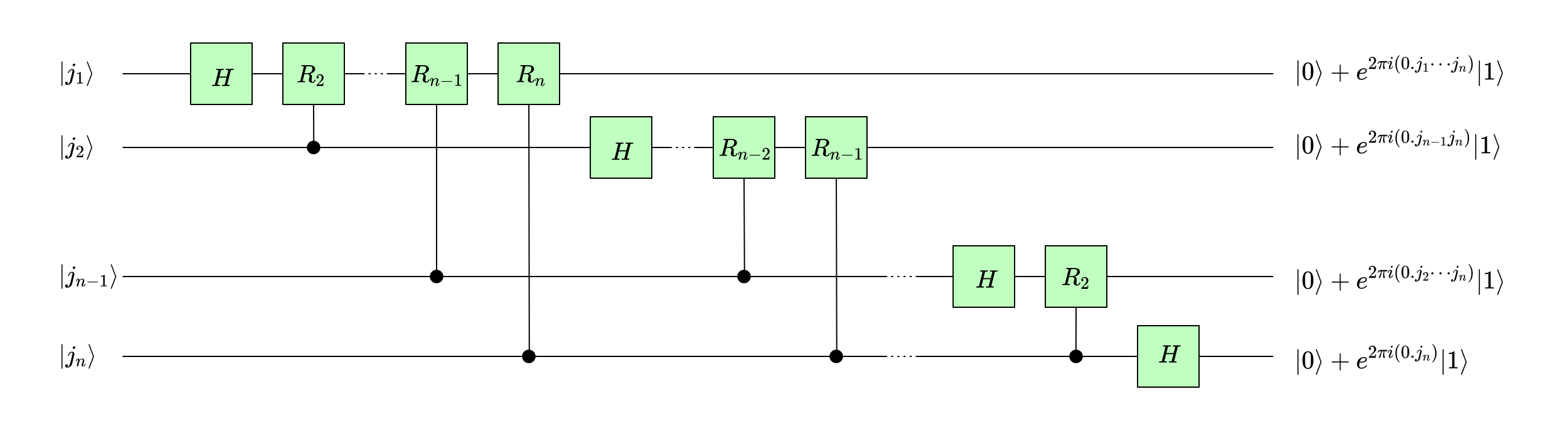
Note we’re omitting the $1/\sqrt{2}$ factor for simplicity.
Reversing bits
The circuit we provided above generates the output in the reverse order, since for example $(\ket{0} + e^{2 \pi i (0.j_n)} \ket{1})$ is constructured from the last bit $j_n$ but it’s the first factor in (8). We can reverse the order of the bits by swapping $N/2$ bits using the 3 CNOT gates we described in Swapping qubits. However, we only showed how to swap bits in the computational base state $\curly{0, 1}$, which the output is not in. The input $\ket{k}$ is, so we can reverse the bits beforehand.
Complexity
We saw that the quantum circuit from the previous section computes the quantum fourier transform. We first need to reverse the bits which can be done in $O(n)$ where $n$ is the number of qubits. Then we have $O(n)$ Hadamard gates and $O(n^2)$ $CR_k$ gates, for a total time complexity of $O(n^2)$ (since each gate can compute in O(1)).
Constrast this with the classical Fourier transform, which is computed in $O(N \log N)$ using the Fast Fourier Transform, FFT. Since $n$ is the number of bits, $N = 2^n$ and the complexity is $O(2^n n)$, which means the quantum circuit is exponentially for efficient.
Note however that similar to the constructs we studied in The Deutsch-Jozsa Algorithm algorithm, this procedure constructs a quantum state that encodes the computed results of the fourier transform but acessing that information is another story. We’ll stop here in this post but will discuss applications in future ones, including prime factorization.
Conclusion
This post are basically my study notes from Chapter 5.1 from Quantum Computation and Quantum Information [1], but with some more details filled in. It was particularly challenging to understand the Step 5 since it implicitly relies on some Euler’s identity properties. It could be this was covered in a previous chapter and I missed it since I’m not reading the book in linear fashion.
The book uses notations I’m not used to and I decide to avoid using them for simplicity. The major example is to represent $y = f(x)$ as $x \rightarrow f(x)$ and omitting $y$ (the book does that for the quantum fourier transform equation).
I assume it wasn’t a clear straight path of discovery from (3) to (8) but I can’t help being astonished by the ingenuity of the logical leaps in there.
Related Posts
- The Deutsch-Jozsa Algorithm besides being the pre-requisite for this post, I noticed similarities between the quantum Fourier transform computation and the Deutsch-Jozsa Algorithm, in which we leverage the ability of quantum circuits to “entangle” information from the input efficiently. In the Deutsch-Jozsa Algorithm, we entangled all the computations of some $f: \curly{\ket{0}, \ket{1}}^{\otimes n} \rightarrow \curly{\ket{0}, \ket{1}}$ while here we entangle all the bits of the input into the each bit of the output, like the last factor of (8) $(\ket{0} + e^{2 \pi i (0.j_1j_2 \cdots j_n} \ket{1})$.
Mentioned by Discrete Fourier Transforms.
References
- [1] Quantum Computation and Quantum Information - Nielsen, M. and Chuang, I.
