kuniga.me > NP-Incompleteness > The Deutsch-Jozsa Algorithm
The Deutsch-Jozsa Algorithm
11 Oct 2020
David Elieser Deutsch is a British scientist at the University of Oxford, being a pioneer of the field of quantum computation by formulating a description for a quantum Turing machine.
Richard Jozsa is an Australian mathematician at the University of Cambridge and is a co-inventor of quantum teleportation.
Together they proposed the Deutsch-Jozsa Algorithm which, although not useful in practice, it provides an example where a quantum algorithm can outperform a classic one.
In this post we’ll describe the algorithm and the basic theory of quantum computation behind it.
Quantum Mechanics Abstracted
In this post we’ll work with abstractions on top of Quantum mechanics concepts, namely qubits and quantum gates. A lot of properties we’ll leverage such as superposition and teleportation arise from the theory of Quantum mechanics but we’ll not delve into their explanation, but rather take them as facts to keep things simpler.
We’ll also try to avoid making real-world interpretations of the theoretical results, since it’s known to be counter-intutive, sometimes paradoxical and overall not agreed upon [1].
The Qubit
We’ll start by defining the quatum analog to a classical bit, which is named a qubit or simply qbit. A common statement about a qubit is that it can be both 0 and 1 at the same time, but as we mentioned in the previous section, we’ll avoid making interpreations such as these and will focus on its mathematical intepretation of a qubit instead.
The Dirac notation defines the pair $\langle \cdot \mid$ and $\mid \cdot \rangle$, called respectively bra and ket (possibly a word play from bracket). A qubit is often represented by the ket symbol: $\ket{\psi}$.
The State of a Qubit
We can think of a qubit as a pair of complex numbers subject to some constraint. More formally, the set of values of a qubit is a vector space represented by the complex linear combination of an orthonormal basis. The orthonormal base used is often $\ket{0}, \ket{1}$, which are also called computational basis states.
In other words, any qubit can be represented as:
\[\ket{\psi} = \alpha \ket{0} + \beta \ket{1}\]where $\alpha$ and $\beta$ are complex numbers and called the amplitude, and $\abs{\alpha}^2 + \abs{\beta}^2 = 1$. It’s worth recalling that the magnitude of a complex number number $c = a + bi$ is $\abs{c} = \sqrt{a^2 + b^2}$, so both $\abs{\alpha}$ and $\abs{\beta}$ are non-negative numbers.
We could have opted to use matrix notation and represent our qubit as:
\[\begin{bmatrix} \psi_{1} \\ \psi_{2} \\ \end{bmatrix} = \alpha \begin{bmatrix} 1 \\ 0 \\ \end{bmatrix} + \beta \begin{bmatrix} 0 \\ 1 \\ \end{bmatrix}\]Multiple Qubits
A state with 2-qubits can be written as:
\[\ket{\psi} = \alpha_{00} \ket{00} + \alpha_{01} \ket{01} + \alpha_{10} \ket{10} + \alpha_{11} \ket{11}\]Note that the size of the base is $2^n$ if $n$ is the number of qubits.
We might also see this notation that factors common terms, so for example the above can be rewritten as:
\[\ket{\psi} = \ket{0} (\alpha_{00} \ket{0} + \alpha_{01} \ket{1}) + \ket{1} (\alpha_{10} \ket{0} + \alpha_{11} \ket{1})\]We can also use multiple variables to represent a multi-qubit, so for example a 2-qubit can be denoted by $\ket{x, y}$ where $\ket{x}$ and $\ket{y}$ are single qubit variables.
Finally, we can represent repeated qubits using the operator $\otimes$, called tensor. For example, the 4-qubit state $\ket{0000}$ can be represented as $\ket{0}^{\otimes 4}$.
Measuring the state of a Qubit
If we measure a single qubit state like
\[\ket{\psi} = \alpha \ket{0} + \beta \ket{1}\]the measurement will return $\ket{0}$ with probability $\abs{\alpha}^2$ and $\ket{1}$ with probability $\abs{\beta}^2$ (recall that $\abs{\alpha}^2 + \abs{\beta}^2 = 1$, so this is a valid probability distribution). One important thing to note is that this process is irreversible, once the measurement is made, the qubit will assume the measured state.
We can also measure partial qubits of a multi-qubit state. Suppose we have a 2-qubit state:
\[\ket{\psi} = \alpha_{00} \ket{00} + \alpha_{01} \ket{01} + \alpha_{10} \ket{10} + \alpha_{11} \ket{11}\]And we measure the first qubit. It will return $\ket{0}$ with probability $\abs{\alpha_{00}}^2 + \abs{\alpha_{01}}^2$ and $\ket{1}$ with probability $\abs{\alpha_{01}}^2 + \abs{\alpha_{11}}^2$. Then the first qubit will assume the measured value. Say we measured $\ket{0}$, then the new state is
\[\ket{\psi} = \frac{\alpha_{00} \ket{00} + \alpha_{01} \ket{01}}{\sqrt{\abs{\alpha_{00}}^2 + \abs{\alpha_{01}}^2}}\]Where the denominator is a normalizing factor so the amplitudes form a valid probability distribution.
Transforming a Qubit: Quantum Gates
In the same way classical gates can be used to transform a bit or bits, we have the analogous quantum gates. The most basic classical gate is the NOT gate which transforms 0 into 1 and vice-versa. The analogous quantum gate flips $\alpha$ and $\beta$ of a state, which is a more general form of a NOT gate, since it also turns $\ket{0}$ into $\ket{1}$ (when $\alpha = 1$, $\beta = 0$) and $\ket{1}$ into $\ket{0}$ (when $\alpha = 0$, $\beta = 1$).
In matricial form, we want to find a transformation from column vector $[\alpha \, \beta]^T$ into $[\beta \, \alpha]^T$. We can do so using a 2 x 2 matrix:
\[\begin{bmatrix} \beta \\ \alpha \\ \end{bmatrix} = \begin{bmatrix} 0 & 1 \\ 1 & 0 \\ \end{bmatrix} + \begin{bmatrix} \alpha \\ \beta \\ \end{bmatrix}\]More generally any quantum gate on $n$-qubits can be represented by a $2^n \otimes 2^n$ matrix called a unitary matrix. A unitary matrix $U$ is such that $U^\dagger U = I$. Where $U^\dagger$ is the adjoint of $U$, which is the result of transposing $U$ and taking conjugate (i.e. negating the imaginary part of the complex number) of the elements.
The Hadamard Gate
The Hadamard gate appears in many constructs and can be defined by:
\[H = \frac{1}{\sqrt{2}}\begin{bmatrix} 1 & 1 \\ 1 & -1 \\ \end{bmatrix}\]Thus if applied on
\[\alpha \ket{0} + \beta \ket{1}\]It yields
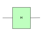
\[\alpha \frac{\ket{0} + \ket{1}}{\sqrt{2}} + \beta \frac{\ket{0} - \ket{1}}{\sqrt{2}}\]The Hadamard gate can be drawn like a classic gate:
The CNOT Gate
The CNOT gate, also known as controlled-NOT, takes two qubits, called control and target. It can be represented by a 4 x 4 matrix:
\[U_{CN} = \begin{bmatrix} 1 & 0 & 0 & 0 \\ 0 & 1 & 0 & 0 \\ 0 & 0 & 0 & 1 \\ 0 & 0 & 1 & 0 \\ \end{bmatrix}\]So for a state given by:
\[\ket{\psi} = \alpha_{00} \ket{00} + \alpha_{01} \ket{01} + \alpha_{10} \ket{10} + \alpha_{11} \ket{11}\]We’ll end up with
\[\ket{\psi} = \alpha_{00} \ket{00} + \alpha_{01} \ket{01} + \alpha_{11} \ket{10} + \alpha_{10} \ket{11}\]Where the 3-rd and 4-th terms got swapped. Let’s consider some special cases.
If the first qubit is $\ket{0}$ (that is, $\alpha_{10} = \alpha_{11} = 0$) then the initial state is
\[\ket{\psi} = \alpha_{00} \ket{00} + \alpha_{01} \ket{01}\]and applying the gate preserves the state. If the first qubit is $\ket{1}$ (that is, $\alpha_{00} = \alpha_{01} = 0$), then the initial state is
\[\ket{\psi} = \alpha_{11} \ket{10} + \alpha_{10} \ket{11}\]and the resulting state is as if the NOT gate had been applied:
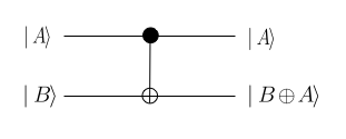
\[\ket{\psi}' = \alpha_{10} \ket{10} + \alpha_{11} \ket{11}\]In other words, the first qubit controls whether the second qubit will be NOTed, hence the name control. In a classical world, this could be achived by the XOR operation between the first and second bits, denoted by the symbol $\oplus$, so the same notation is used to represent the result of the second qubit.
Summarizing, if we’re given qubits $\ket{x, y}$, this gate returns $\ket{x, x \oplus y}$:
Quantum Circuits
A quantum circuit is simply a composition of one or more quantum gates, analogous to a classical circuit.
Quantum Parallelism
Suppose we have a gate, which we’ll call $U_f$, that transforms a 2-qubit state $\ket{x,y}$ into $\ket{x, y \oplus f(x)}$ where $f(x)$ is any function that transforms a qubit into a $\ket{0}$ or $\ket{1}$ (i.e. a computational basis state) and $\oplus$ the XOR operator as defined in the CNOT gate. We’ll treat it as a blackbox but it can be shown to be a valid quantum gate (i.e. it has a corresponding unitary matrix transformation).
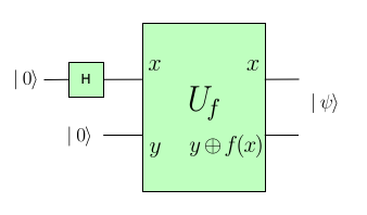
Say $\ket{x} = \frac{\ket{0} + \ket{1}}{\sqrt{2}}$ and $\ket{y} = \ket{0}$, where the state $\ket{x}$ can be obtained by applying the Hadamard gate over $\ket{0}$. Then the resulting state will be
\[\frac{\ket{0, f(0)} + \ket{1, f(1)}}{\sqrt{2}}\]This is interesting because it contains the evaluation of $f(x)$ for both values $\ket{0}$ and $\ket{1}$.
We can generalize $\ket{x}$ to have $n$ qubits and apply the Hadamard gate to each of them, which can be denoted as $H^{\otimes n}$. For $n = 2$ if we apply $H^{\otimes 2}$ to $\ket{00}$ we get:
\[\bigg( \frac{\ket{0} + \ket{1}}{\sqrt{2}} \bigg) \bigg( \frac{\ket{0} + \ket{1}}{\sqrt{2}} \bigg) = \frac{\ket{00} + \ket{01} + \ket{10} + \ket{11}}{2}\]In general it’s possible to show that if we apply $H^{\otimes n}$ to $\ket{0}^{\otimes n}$ we get:
\[H^{\otimes n}(\ket{0}^{\otimes n}) = \frac{1}{\sqrt{2^n}} \sum_x \ket{x}\]Where $x$ is all binary numbers with $n$ bits.
Going back to our original gate $U_f$, if we set $\ket{x} = H^{\otimes n}(\ket{0}^{\otimes n})$, we’ll get the state
\[\frac{1}{\sqrt{2^n}} \sum_x \ket{x} \ket{f(x)}\]The insight is that we now have a state encoding $2^n$ values of $f(x)$ and we achieved that using only $O(n)$ gates. Unfortunately as we saw in Measuring the state of a Qubit, there’s no way to extract all these values from a quantum state, and once we perform a measurement only one of the values of $x$ will be returned.
We’ll see next how to “entagle” these values such that any measurement will result in a value resulting from computing $f(x)$ for all values of $x$.
The Deutsch Algorithm
The Deutsch Algorithm is a more complex circuit using the $U_f$ gate from the previous session, which involves applying the Hadamard gate to both input qubits and then to the first qubit of the output:
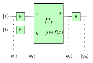
Let’s follow the state at each step of the circuit:
\[\ket{\psi_0} = \ket{01}\]Applying the Hadamard gate to each of the qubits:
\[\ket{\psi_1} = \bigg[ \frac{\ket{0} + \ket{1}}{\sqrt{2}} \bigg] \bigg[ \frac{\ket{0} - \ket{1}}{\sqrt{2}} \bigg]\]Let’s assume $\ket{x} = \frac{\ket{0} + \ket{1}}{\sqrt{2}}$ and $\ket{y} = \frac{\ket{0} - \ket{1}}{\sqrt{2}}$.
Now, what is the result of applying $U_f$ over $\ket{\psi_1}$? First let’s assume the first qubit is either $\ket{0}$ or $\ket{1}$ (i.e. a computational basis). Now suppose $f(x) = \ket{0}$. Then $f(x) \oplus y = y$ and $U_f$ will yield the same state $\ket{x} \ket{y}$. If $f(x) = \ket{1}$, then $f(x) \oplus y$ is $y$ with its terms flipped, which in this particular case is $-y$, so in general we have:
\[U_f(\ket{x} \ket{y}) = (-1)^{f(x)} \ket{x} \ket{y}\]However, $\ket{x}$ is not in a computational base state, but we can use the linearity principle when applying a function over a quantum state, that is:
\[f(\ket{x}) = f(\alpha \ket{0} + \beta \ket{1}) = \alpha f(\ket{0}) + \beta f(\ket{1})\]Since $\ket{x} = \frac{\ket{0} + \ket{1}}{\sqrt{2}}$ the output of $U_f(\ket{x} \ket{y})$ is
\[U_f(\ket{x} \ket{y}) = \frac{(-1)^{f(\ket{0})} \ket{0} + (-1)^{f(\ket{1})} \ket{1}}{\sqrt{2}} \ket{y}\]We can group the results in two cases: one where $f(\ket{0}) = f(\ket{1})$, in which case $(-1)^{f(\ket{0})}$ and $(-1)^{f(\ket{1})}$ have the same sign, say $z = \pm 1$:
\[U_f(\ket{x} \ket{y}) = \frac{z \ket{0} + z \ket{1}}{\sqrt{2}} \ket{y} = \pm \frac{\ket{0} + \ket{1}}{\sqrt{2}} \ket{y} = \pm \ket{x} \ket{y}\]another wwhere $f(\ket{0}) \neq f(\ket{1})$ when $(-1)^{f(\ket{0})}$ and $(-1)^{f(\ket{1})}$ have opposite signs, so say $(-1)^{f(\ket{0})} = z$ and $(-1)^{f(\ket{0})} = -z$:
\[U_f(\ket{x} \ket{y}) = \frac{z \ket{0} - z \ket{1}}{\sqrt{2}} \ket{y} = \pm \frac{\ket{0} - \ket{1}}{\sqrt{2}} \ket{y} = \pm \ket{\bar x} \ket{y}\]Where we define $\ket{\bar{x}} = \frac{\ket{0} - \ket{1}}{\sqrt{2}}$, that is, it’s $\ket{x}$ with the sign of $\ket{1}$ negated.
Summarizing,
\[\ket{\psi_2} = \begin{cases} \pm \ket{x}\ket{y} & \text{if } f(0) = f(1) \\ \pm \ket{\bar x}\ket{y}, & \text{if } f(0) \neq f(1) \end{cases}\]To compute $\ket{\psi_3}$ we just need to apply the Hadamard gate on the firt qubit. We can show that $\ket{H(x)} = \ket{0}$ and $\ket{H(\bar x)} = \ket{1}$, so:
\[\ket{\psi_3} = \begin{cases} \pm \ket{0}\ket{y} & \text{if } f(0) = f(1) \\ \pm \ket{1}\ket{y}, & \text{if } f(0) \neq f(1) \end{cases}\]This can be further compacted by noting $\ket{f(0) \oplus f(1)} = \ket{0}$ if $f(0) = f(1)$ and $\ket{f(0) \oplus f(1)} = \ket{1}$ otherwise:
\[\ket{\psi_3} = \ket{f(0) \oplus f(1)}\ket{y}\]This also makes it clearer that if we measure the first qubit, regardless of the result, it has to have computed both $f(0)$ and $f(1)$. We don’t have access to the individual values of the function evaluations, but we can access the result of a computation that evaluated $2$ functions in one operation. This gain will be more obvious next where we generalize this to $n$ qubits.
The Deutsch-Jozsa Algorithm
The Deutsch-Jozsa Algorithm is a generalization of the Deutsch for $n$-qubits. The circuit is almost exactly the same:
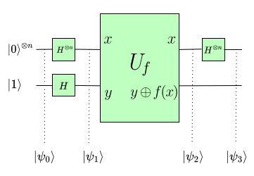
The difference is that instead of one qubit for the state on top, we generalize to $n$-qubits. Let’s analyze the state at each step of the circuit:
\[\ket{\psi_0} = \ket{0}^{\oplus n} \ket{1}\]Applying a Hadamard gate to $\ket{0}^{\oplus n}$ yields $\frac{1}{\sqrt{2^n}} \sum_x \ket{x}$ as we saw in Quantum Parallelism, so $\ket{\psi_1}$ is:
$\ket{\psi_1} = \frac{1}{\sqrt{2^n}} \sum_x \ket{x} \ket{y}$
Where $\ket{y} = \frac{\ket{0} - \ket{1}}{\sqrt{2}}$ as in the Deutsch Algorithm. Let’s call $\ket{X} = \frac{1}{\sqrt{2^n}} \sum_x \ket{x}$.
As we saw in the previous session, if we assume $x$ in some computation basis state, then
\[U_f(\ket{x} \ket{y}) = (-1)^{f(x)} \ket{x} \ket{y}\]This remains true for any number of qubits because both $f(\ket{x})$ and $\ket{y}$ are still one qubit. Leveraging the linearity of terms in $\ket{X}$ we have
\[\ket{\psi_2} = U_f(\ket{X} \ket{y}) = \frac{1}{\sqrt{2^n}} \sum_x U_f(\ket{x} \ket{y}) = \frac{1}{\sqrt{2^n}} \sum_x (-1)^{f(x)} \ket{x} \ket{y}\]Let’s define
\[\ket{X_2} = \frac{1}{\sqrt{2^n}} \sum_x (-1)^{f(x)} \ket{x}\]We now need to apply the Hadamard gate to $\ket{X_2}$. We know how to compute the Hadamard gate for $\ket{0}^{\oplus n}$, but let’s see how to do this for an arbitrary computation basis state. To get an intuition, we can try to find a pattern for 1-qubit:
\[H(\ket{0}) = \frac{\ket{0} + \ket{1}}{\sqrt{2}}\] \[H(\ket{1}) = \frac{\ket{0} - \ket{1}}{\sqrt{2}}\]They look very similar except for the signs on $\ket{1}$, if we could parametrize that sign based on the input and which term from the output we’re at, this could be succintly represented as a summation. Turns out it’s possible: let $z$ be a computation basis state from the output (that is, $\ket{0}$ and $\ket{1}$). If we define the term $(-1)^{xz} \ket{z}$, we can show that
\[H(\ket{x}) = \sum_{z} \frac{(-1)^{xz} \ket{z}}{\sqrt{2}}\]It’s possible to generalize this to $n$-qubits:
\[H^{\otimes n}(\ket{x}) = \sum_{z} \frac{(-1)^{x \cdot z} \ket{z}}{\sqrt{2^n}}\]Where $x \cdot z$ is the inner product modulo 2. Again, this assumes $\ket{x}$ is in a computation basis state. Our $\ket{X_2}$ is not, but its terms are, so we can simply use the linearity principle:
\[H^{\otimes n}(\ket{X_2}) = \frac{1}{\sqrt{2^n}} \sum_x (-1)^{f(x)} H^{\otimes n} (\ket{x}) = \frac{1}{2^n} \sum_x (-1)^{f(x)} \sum_z (-1)^{x \cdot z} \ket{z}\]We can exchange the summation over $x$ with that of $z$ for a cleaner form:
\[H^{\otimes n}(\ket{X_2}) = \frac{\sum_z \sum_x (-1)^{x \cdot z + f(x)} \ket{z}}{2^n}\]Using this, we can finally compute the final state of the circuit:
\[\ket{\psi_3} = \frac{\sum_z \sum_x (-1)^{x \cdot z + f(x)} \ket{z}}{2^n} \ket{y}\]If we measure the state of the first $n$-qubits, we’ll obtain the term for a given $z$, say $\frac{\sum_x (-1)^{x \cdot z + f(x)} \ket{z}}{\sqrt{2^n}}$ and that contains a computation involving all the $2^n$ computational base states, and we did so with only $O(n)$ operations!
What can we do with this? We’ll next present a contrived problem which can be solved using this result.
The Deutsch’s Problem
The Deutsch can be described as follows: let $f(x)$ be a function that takes a $n$-bit number and return true or false. It can be either a constant function, one that returns true (or false, but not both) for all its inputs, or a balanced function, which returns true for exactly half of it’s input.
To be super clear, an example of a constant function is:
def constant(x):
    return true
An example of a balanced function is:
def balanced(x):
    return x % 2
It’s easy to tell which type of functions the examples above are, but in general, we’d need to evaluate a function for at least the majority of all the possible inputs, that is $2^n/2 + 1$, which would make this classication process an exponential one using a classical computer.
For a quantum computer, we can assume we used $U_f$ and have the state:
\[\ket{\psi_3} = \frac{\sum_z \sum_x (-1)^{x \cdot z + f(x)} \ket{z}}{2^n} \ket{y}\]Let $\ket{X_3}$ be the non-$y$ part of this state:
\[\ket{X_3} = \frac{\sum_z \sum_x (-1)^{x \cdot z + f(x)} \ket{z}}{2^n}\]Suppose we performed a measurement on the qubit and got the state $z = \ket{0}^{\otimes n}$. The correspond amplitude of this state is
\[\alpha_{0^{\otimes n}} = \frac{\sum_x (-1)^{x \cdot z + f(x)}}{2^n} = \frac{\sum_x (-1)^{f(x)}}{2^n}\]The last step comes from $x \cdot \vec{0} = 0$, and the probability of getting that state is $\abs{\alpha_{0^{\otimes n}}}^2$.
Now suppose $f(x)$ is constant and always returns $k$. Then
\[\alpha_{0^{\otimes n}} = (-1)^k \frac{\sum_x 1}{2^n} = (-1)^k \frac{2^n}{2^n} = \pm 1\]This means that if $f(x)$ is constant, then $\abs{\alpha_{0^{\otimes n}}}^2 = 1$ and since the sum of the square of amplitudes must be 1, this means the other amplitues are 0, and we’ll obtain state $z = \ket{0}^{\otimes n}$ with 100% probability.
Now suppose $f(x)$ is balanced. Then half of the terms in $\sum_x (-1)^{f(x)}$ will be positive ($f(x) = 0$), and half negative ($f(x) = 1$), so the $\alpha_{0^{\otimes n}} = 0$ and the probability of obtaining $z = \ket{0}^{\otimes n}$ is 0.
This gives a simple proxy to determine whether $f(x)$ is constant or balanced. If we measure $\ket{X_3}$ and get $\alpha_{0^{\otimes n}}$, the function is constant, otherwise it’s balanced, and we determined this in $O(n)$ operations as opposed to thr $O(2^n)$ of a classical computer.
Conclusion
In this post we covered the Deutsch-Jozsa Algorithm, which on one hand provides an example in which a quantum computation outperforms a classical one, but on the other hand it’s simple enough that it requires only the basics of quantum computing to be understood, which allowed for a self-contained post.
I started learning quantum computing via Michael Nielsen’s Youtube videos [3]. Though the series was never finished, he also wrote a book with Issac Chuang, Quantum Computation and Quantum Information, which seems very thorough and well praised, so I’m going to use that for my education.
Here are some difficulties I encountered so far. One is getting used to the notation: I think I get the idea of the ket operator, but it’s still not natural to remember when to wrap variables inside it. I also found it important to be aware of when the state of a qubit has to be in a computation basis or it can be in a more general state. The book seems to be switching between these two types of state implicitly at times and is hard to follow at first.
