kuniga.me > NP-Incompleteness > Amortization and Persistence via Lazy Evaluation
Amortization and Persistence via Lazy Evaluation
19 Mar 2017

In this chapter Okasaki works around the problem of doing amortized analysis with persistent data structures because the amortized analysis assumes in place modification while for persistent data structures (partial) copies are made. The intuition is that lazy evaluation, which comes with memoization and avoids recomputation, solves this problem.
He adapts the Banker’s and Physicists’s methods to work with lazy evaluated operations and applies them to a few structures including Binomial Heaps, Queues and Lazy Pairing Heaps. In this post we’ll only cover the examples of the Queues using both methods.
We’ll first introduce some concepts and terminology, then we’ll present a queue implementation using lazy evaluation that allows us analyzing it under persistence. Following that we’ll explain the Banker’s and Physicist’s methods and prove that the implementation for push/pop has an efficient amortized cost.
Persistence as a DAG
An execution trace is a DAG where nodes represent the operations (e.g. updates to a data structure) and an edge from nodes \(v\) to \(v'\) indicates that the operation corresponding to \(v'\) uses the output of the one corresponding to \(v\).
For example, if we have this set of operations:
let a = push 0 newEmpty
let b = push 1 a
let c = pop b
let d = push 2 b
let e = append c d
let f = pop c
let g = push 3 d
The corresponding execution graph is:
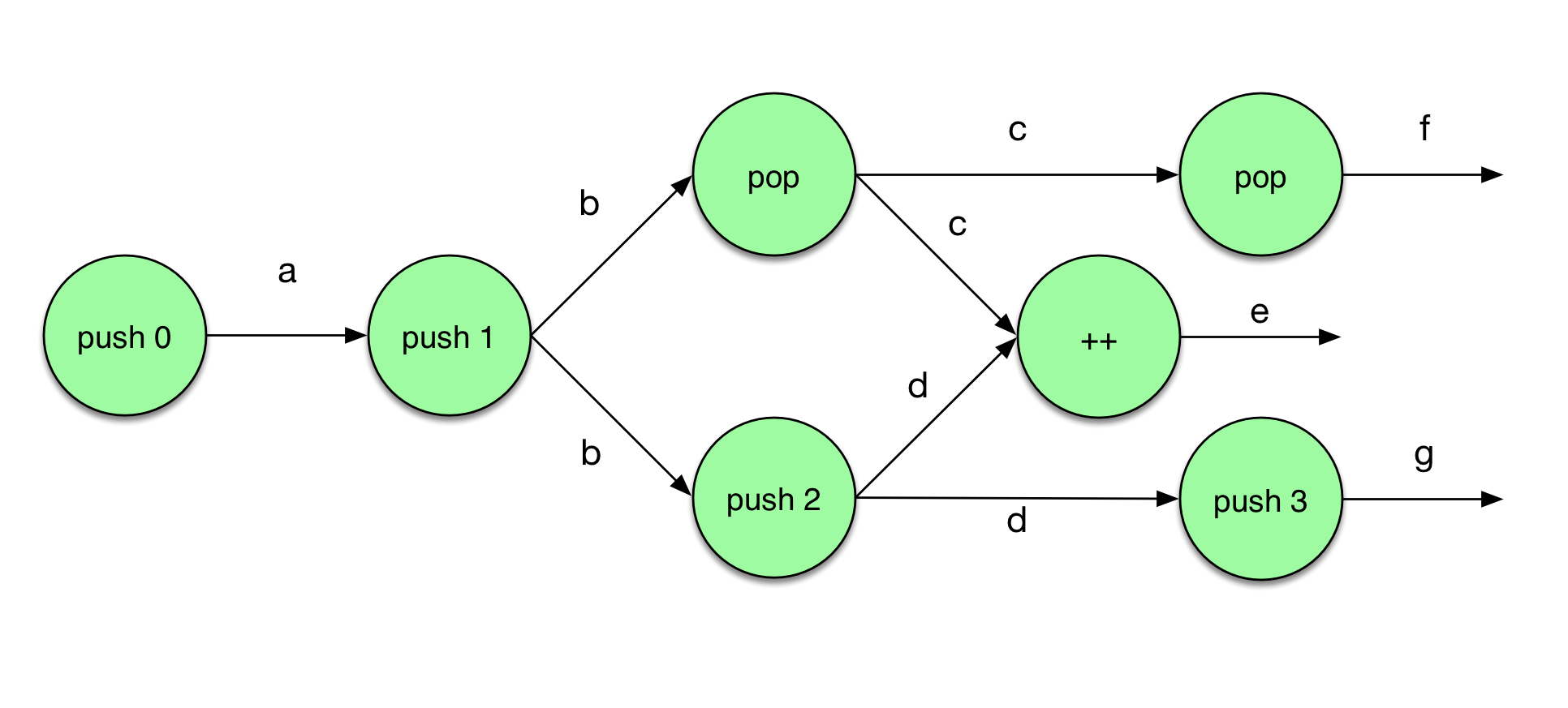
The logical history of an operation v is the set of all operations it depends on (directly or indirectly, and including itself). Equivalently, in terms of the DAG, it’s the set of nodes that have a directed path to v.
A logical future of an operation v is any directed path from v to a terminal node.
A framework for analyzing lazy evaluated data structures
We need to introduce a few more concepts and terminology. Note: we’ll use suspension and lazy operation interchangeably, which can be evaluated or forced.
The unshared cost of an operation is the time it would take to execute it if it had already been performed and memoized before, so if the operation involves any expression that is lazy, that expression would be O(1).
The shared cost of an operation is the time it would take it to execute (force) all the suspensions created (but not evaluated) by the operation.
The complete cost is the sum of the shared and unshared costs. Alternatively, the complete cost of an operation is the time it would take to execute the operation if lazy evaluation was replaced by strict. To see why, first we note that the unshared costs have to be paid regardless of laziness. Since we’re assuming no laziness, the operation has to pay the cost associated with the suspension it creates, which corresponds to the shared costs. Note that under this assumption we wouldn’t need to account for the cost of forcing suspensions created by previous operations because in theory they have already been evaluated.
When talking about a sequence of operations, we can break down the shared costs into two types: realized and unrealized costs. The realized costs are the shared costs from suspensions were actually forced by some operation in the sequence. Example: say that operations A and B are in the sequence and A creates a suspension, and then B forces it. The cost for B to force it is included in the realized cost. The unrealized costs are the shared costs for suspensions that were created but never evaluated within the sequence. The total actual cost of a sequence of operations is the sum of the realized costs and the unshared costs.
Throughout a set of operations, we keep track of the accumulated debt, which starts at 0 at the beginning of the sequence. Whenever an operation is performed, we add its shared cost to it. For each operation, we can decide how much of this debt we want to pay. When the debt of a suspension is paid off, we can force it. The amortized cost of an operation is its unshared cost plus the amount of debt it paid (note that it does not include the realized cost). Note that as long as we always pay the cost of a suspension before it’s forced, the amortized cost will be an upper bound on the actual cost.
This framework simplifies the analysis for the case when a suspension is used more than once by assuming that its debt was paid off within the logical history of when it was forced, so we can always analyze a sequence of operations and don’t worry about branching. This might cause the debt being paid multiple times, but it simplifies the analysis.
The author uses the term discharge debit as synonym of pay off debt. I find the latter term easier to grasp, so I’ll stick with it throughout this post.
Let’s introduce an example first and then proceed with the explanation of the Physicist’s method and the corresponding analysis of the example.
The Stream Queue
To allow efficient operations on a queue in the presence of persistence, we can make some of the operations lazy. Recall in a previous post we defined a queue using two lists. To avoid immediate computation, a natural replacement for lists is using its lazy version, the stream data structure, which we also talked about in a previous post.
For the list-based queue, the invariant was that if the front list is empty, then the rear list must be empty as well. For the stream queue, we have a tighter constraint: ‘front’ must be always greater or equal than ‘rear’. This constraint is necessary for the analysis.
The definition of the stream queue is the following:
(*
  - size of front stream
  - stream representing the front of the queue
  - size of rear stream
  -  stream representing the (reversed) rear of the queue
*)
type 'a queueStream = int * 'a stream * int * 'a stream;;
We store the lengths of the streams explicitly for efficiency.
We’ll be using the Stream developed in the previous chapter, so we’ll refer to the module Stream2 to avoid ambiguity with the standard Stream module.
Inserting an element at the end of the queue is straightforward, since the rear stream represents the end of the queue and is reversed:
let push (elem: 'a) (queue: 'a queueStream): ('a queueStream) = match queue with
  (frontSize, front, rearSize, rear) ->
    check (frontSize, front, rearSize + 1, Stream2.insert elem rear)
;;
The problem is that inserting at rear can cause the invariant of the queue to be violated. check() changes the structure so to conform to the invariant by potentially reversing rear and concatenating with front:
let check (queue: 'a queueStream): ('a queueStream) = match queue with
  (leftSize, left, rightSize, right) ->
    if rightSize <= leftSize then queue
    else (leftSize + rightSize, Stream2.concat left (Stream2.reverse right), 0, Stream2.empty)
;;
Removing an element from the queue requires us to evaluate the first element of the front stream. Again, the invariant can be violated in this case so we need to invoke check() again:
let pop (queue: 'a queueStream): ('a queueStream) = match queue with
  (leftSize, left, rightSize, right) ->
    let forcedLeft = Lazy.force left in
    match forcedLeft with
      | Nil -> raise Empty_queue
      | StreamCell (_, rest) -> check (leftSize - 1, rest, rightSize, right)
;;
The complete code for the stream queue is on Github.
Analysis using the Banker’s Method
The idea of the Banker’s Method is basically define an invariant for the accumulated debt and a strategy for paying it off (that is, decide how much debt each operation pays off). Then we show that whenever we need to force a suspension, the invariant guarantees that the accumulated debt has been paid off. One property of the Banker’s method is that it allows associating the debt to specific locations of the data structure. This is particularly interesting for streams, because it contains multiple (nested) suspensions, so we might force parts of this structure before we paid the debt associated with the entire structure.
By inspection, we can see that the unshared cost of both push and pop are O(1). It’s obvious in the case of push, and in the case of pop, in theory check could take O(m) where m is the size of the queue, but since Stream2.concat() and Stream2.reverse() are both lazy, and hence memoized, they are not included in the unshared costs.
To show that the amortized cost of both operations is O(1), we can show that paying off O(1) debt at each operation is enough to pay for the suspension before it is forced. For the queue, we also need to associate the debt with parts of the data structure, so that we could force the suspension of only some parts of it (for example, on the stream we can evaluate only the head, not necessarily the entire structure).
We now define an invariant that should be respected by all operations. Let \(d(i)\) be the debt at the i-th node on the front stream, and \(D(i) = \sum_{j=0}^{i} d(j)\) the accumulated debt up to node \(i\). The invariant is:
\[D(i) \le \min(2i, \mid f \mid - \mid r \mid)\]This constraint allows us evaluating the head at any time, because \(D(0) = 0\), which means its debt has been paid off. The second term in min(), guarantees that if \(\mid f \mid = \mid r \mid\) the entire stream can be evaluated, because \(D(i) = 0\) for all \(i\).
The author then proves that by paying off one debt in push() and two debt units in pop() is enough to keep the debt under the constraint.
Queue with suspended lists
Because the Physicist’s method cannot assign costs to specific parts of the data structure, it doesn’t matter if the structure can be partially forced (like streams) or if it’s monolithic. With that in mind, we can come up with a simpler implementation of the queue by working with suspended lists instead of streams. Only the front list has to be suspended because the cost we want to avoid, the reversal of the back list and concatenation to the front list, happens on the front list.
On the other hand, we don’t want to evaluate the front list when we perform a peek or pop, so we keep a evaluated version of the front list too.
The signature of the structure is as follows:
(*
    Implemention of queue using lazy lists. As opposed to the stream-based
    queue, this structure allows for a monolithic amortization analysis, for
    example, using the Physicist's method as described in Okazaki's Purely
    Functional Data Structures, Chapter 6.

    Only the front list needs to be lazy. The rear of the queue is a regular
    list. We store a copy of the suspended list to be able to access the head of
    the list without having to evaluate the entire list.

    The first element in the structure is the evaluated version of the front
    (forcedFront). The second represents the size of the front list (frontSize).
    The third element is the suspended version of the front (lazyFront). The
    fourth element is the size of the rear list (rearSize) and finally the fifth
    element is the rear list (rear).

    The invariants that must be respected by all operations are:
    1) The front list must never be smaller than the rear list
    2) Whenever lazyFront is non-empty, forcedFront is non-empty
*)
type 'a queueSuspended = 'a list * int * ('a list) Lazy.t * int * 'a list;;
As mentioned in the code above, the invariants we want to enforce is that the front list is never smaller than the rear list
let conformToFrontNotSmallerThanRear (
  queue: 'a queueSuspended
): ('a queueSuspended) = match queue with
  (forcedFront, frontSize, lazyFront, rearSize, rear) ->
    if rearSize <= frontSize then queue
    else
      let front = Lazy.force lazyFront
      in (
        front,
        frontSize + rearSize,
        lazy (front @ (List.rev rear)),
        0,
        []
      )
;;
and that the evaluated version of the front list is never empty if the lazy version still has some elements.
let conformToForcedFrontInvariant (
  queue: 'a queueSuspended
): ('a queueSuspended) = match queue with
  | ([], frontSize, lazyFront, rearSize, rear) ->
    (Lazy.force lazyFront, frontSize, lazyFront, rearSize, rear)
  | queue -> queue
;;
The push and pop operations are similar to the other versions of queue, but since we mutate the structure, we might need to adjust it to conform to the invariants:
let conformToInvariants (queue: 'a queueSuspended): ('a queueSuspended) =
  let queue = conformToFrontNotSmallerThanRear queue
  in conformToForcedFrontInvariant queue
;;

let push (queue: 'a queueSuspended) (elem: 'a): ('a queueSuspended) =
  match queue with (forcedFront, frontSize, lazyFront, rearSize, rear) ->
    conformToInvariants (
      forcedFront,
      frontSize,
      lazyFront,
      rearSize + 1,
      elem :: rear
    )
;;

let pop (queue: 'a queueSuspended): ('a queueSuspended) = match queue with
  | ([], _, _, _, _) -> raise Empty_queue
  | (head :: forcedFront, frontSize, lazyFront, rearSize, rear) ->
      conformToInvariants (
        forcedFront,
        frontSize - 1,
        lazy (List.tl (Lazy.force lazyFront)),
        rearSize,
        rear
        )
;;
Finally, because of our second invariant, peeking at the queue is straightforward:
let peek (queue: 'a queueSuspended): 'a = match queue with
  | ([], _, _, _, _) -> raise Empty_queue
  | (head :: forcedFront, _, _, _, _) -> head
;;
The complete code for the suspended queue is on Github.
Analysis using the Physicist’s Method
We’ve seen the Physicist’s Method in a previous post when we’re ignore the persistence of the data structures. We adapt the method to work with debits instead of credits. To avoid confusion, we’ll use \(\Psi\) to represent the potential function. \(\Psi(i)\), represents the accumulated debt of the structure at step \(i\). At each operation we may decide to pay off some debit, which will be then included in the amortized cost. We have that \(\Psi(i) - \Psi(i - 1)\) is the increase in debt after operation \(i\). Remember that the shared cost of an operation corresponds to the increase in debt if we don’t pay any of the debt. Thus, we can find out how much debt was paid off then by \(s_i - \Psi(i) - \Psi(i - 1)\), where \(s(i)\) is the shared costs of operation \(i\). Let \(u(i)\) and \(c(i)\) be the unshared and complete costs of the operation \(i\). Given that, by definition, \(c(i) = u(i) + s(i)\), we can then express the amortized cost as:
\[a_i = cc_i - (\Psi(i) - \Psi(i - 1))\]To analyze the suspended queue we need to assign values to the potentials such that by the time we need to evaluate a suspension the potential on the structure is 0 (that is, the debt has been paid off). For the suspended queues we’ll use the following potential function:
\[\Psi(q) = \min(2\mid w \mid, \mid f \mid - \mid r \mid)\]Where w is the forcedFront, f is lazyFront and r is rear.
We now claim that the amortized cost of push is at most 2. If we push and element that doesn’t cause a rotation (i.e. doesn’t violate \(\mid f \mid \ge \mid r \mid\)), then \(\mid r \mid\) increases by 1, and the potential decreases by 1. No shared is incurred and the unshared cost, inserting an element at the beginning of rear is 1, hence the amortized cost for this case is 1 - (-1) = 2. If it does cause a rotation, then it must be that after the insertion \(\mid f \mid = m\) and \(\mid r \mid = m + 1\). After the rotation we have \(\mid f \mid = 2*m + 1\) and \(\mid r \mid = 0\), but w hasn’t changed and cannot be larger than the original \(f\), so the potential function is at most \(2*m\). The reversal of \(r\) costs \(m + 1\) and concatenating to a list of size \(x\) costs \(x\) (discussed previously), plus the cost of initially appending an element to read, so the unshared cost is \(2*m + 2\). No suspensions were created, so the amortized cost is given by \(2*m + 2 - (2*m) = 2\).
Our next claim is that the amortized cost of pop is at most 4. Again, if pop doesn’t cause a rotation, \(\mid w \mid\) decreases by 1, so the potential is reduced by 2. The unshared cost is 1, removing an element from \(w\), and the shared cost, 1 comes from the suspension that lazily removes the head of lazyFront. The amortized cost is 2 - (-2) = 4. Note that if \(w = 0\), we’ll evaluate \(f\), but the ideas is that it has been paid off already. If the pop operation causes a rotation, then the analysis is similar to the push case, except that the complete cost is must account for the shared cost of lazily reming the head of lazyFront, so it’s \(2*m + 3\), for an amortized cost of 3.
Note that when the suspensions are evaluated, the potential is 0, either when \(\mid f \mid = \mid r \mid\) or \(\mid w \mid = 0\).
Conclusion
In this post we covered a simple data structure, the queue, and modified it to be lazy evaluated and can show, with theory, that it allows for efficient amortized costs. The math for proving the costs is not complicated. The hardest part for me to grasp is to get the intuition of how the analysis works. The analogy with debt is very useful.
Meta: Since wordpress code plugin doesn’t support syntax highlighting for OCaml, I’m experimenting with the Gist plugin. Other advantages is that Gists allow comments and has version control!
