kuniga.me > NP-Incompleteness > Persistent Data Structures

Persistent Data Structures

23 Oct 2016

In this post we’ll discuss some basic data structures in functional programming and their implementation in OCaml. Our main reference are the first two chapters of Purely Functional Data Structures by Chris Okasaki.

The first chapter explains persistent data structures and the second chapter provides examples of three common data structures in imperative programming and how to implement them in ML (a functional language).

Persistent Data Structures

The core idea behind designing data structures in functional languages is that they’re immutable, that is, if you want to modify it, a new copy has to be made.

If we want to modify a data structure in the naive way, we would need to clone the entire structure with the modifications. Instead, this is done in a smart way so different versions of the data structure share them. Two examples are given to illustrate this idea: lists and binary trees.

Immutable Linked Lists

Lists are a central native data structure in functional languages. In Ocaml, they’re implemented as linked list. From our data structure class, we know that inserting an element at the beginning of a list is an O(1) operation, but this requires modifying pointers in the data structure. As we said data structures are immutable, so we need to make a copy to perform this operation.

Note that we only need to make the new node point to the beginning of the original list, which means we don’t have to clone this list, we just reuse it.

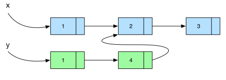
Now, if we’re inserting in the middle of the list will require copying the existing nodes until we reach our newly inserted element, which we can then point to the remaining of the original list. Consider the example below, where we insert the element 4 in the second position of the list.

Note that inserting an element at the beginning of a linked list is much more efficient than at the end, both in terms of complexity and space. If we were to insert it at the end, we would require full copies and insertion would be O(length of the list). As an experiment, we can write a function that generates a list representing a range of integers in two ways.

In example 1, we create the list by inserting an element at the beginning of the array,

let rec list_range_fast start_range end_range =
  if start_range == end_range then []
  else start_range :: (list_range_fast (start_range + 1) end_range)
;;

In example 2 we do it at the end:

let rec list_range_slow start_range end_range =
  if start_range == end_range then []
  else (list_range_slow start_range (end_range - 1)) @ [end_range]
;;

If I run the slow version with start_range = 0 and end_range = 50000, it takes over a minute to run on my computer, while the fast version runs in a few milliseconds.

Immutable Binary Trees

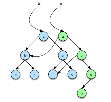
Binary trees are a generalized version of a linked list and it works the same way. The key point to notice is that when inserting an element in a (binary) tree only the nodes in the path from the root to the inserted node need to have their pointers modified, so we need to clone a number of nodes that are at most the height of the tree. See the example below:

With this basic concept understood for simple constructs like linked lists and binary trees, we can construct basic data structures on top of them: heaps and balanced binary trees.

Leftist Heaps

A (minimum) leftist heap is a binary tree with the following properties:

1. The value of a node is smaller or equal the value of its children.

Let the spine of a node be the path defined by following the right children until a leaf is found (i.e. the rightmost path), and the rank of a node the length of its spine.

1. The rank of the left child is always greater or equal than the right child.

It’s possible to show that the rank of a heap of n nodes is less or equal than O(floor(log n + 1)).

Insertion. Before talking about inserting an element in a heap, let’s define the more general merge() function, which merges two leftist heaps, A and B, into one. We compare the root of each heap, say A.val and B.val. If A.val <= B.val, we make A.val the root of the new heap, A.left the left of the new heap and the right of the new heap will be the merge of A.right and B. If A.val >= B.val we do an analogous operation.

Note that the result of the merge might violate property 2, since we’re adding a new node to the right subtree. This is easy to fix: we just to swap the left and right subtree when coming back from the recursion. This is what makeTree() does.

Note that we always perform the merges of the right, which means that the number of such merges will be proportional to the largest rank the original heaps, which implies we can do it in O(log(A.size + B.size)).

In the context of immutable structures, this implementation of heap is efficient because the only nodes whose pointers we need to mutate (even when a swap is needed) are on the spine of the trees, so it only needs to create O(log n) new nodes.

The insertion process consists in creating a heap with one element and merging into the target heap.

Returning the minimum element is trivial: we just need to return the element at the root. Removing the minimum is easy as well: just merge the left and right subtree using merge().

My implementation for the leftist heap is on github.

Binomial Heaps

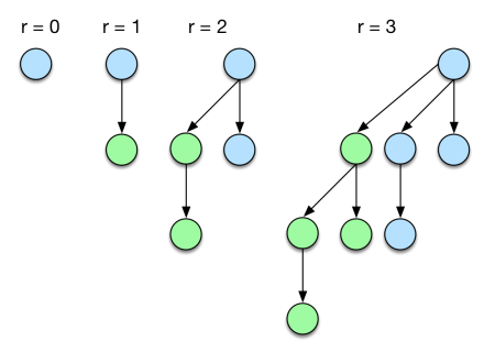
Binomial heaps are an alternative heap implementation. Before defining a binomial heap, let’s introduce the binomial tree. A binomial tree is a can be defined recursively based on a property called rank. A single node is a binomial tree of rank 0. A tree of rank r > 0, is formed by combining two trees of rank r-1 making one tree the leftmost child of the other. We denote this operation as linking.

A binomial heap is a list of binomial trees ordered by increasing rank, with no trees with the same rank.

Insertion. Before talking about insertion of an element into a heap, let’s see how to insert a binomial tree of rank r into the heap. To keep the order of the rank of the tree list, we need to traverse through it to find the right place to insert it. Since we can’t have two trees with the same rank, if we run into this case we need to merge those two trees into one with rank r + 1. This can cascade so we might need to repeat this process with the new tree.

Linking a tree is a direct application of its definition. We just need to decide which of the trees will become child of the other. Since we want a minimum heap, we need to guarantee that the minimum element is always on top, so we always make the tree with smallest root to be on top.

Linking is a constant time operation, since we only need to update the pointer of the root of the top tree, which also means we only need to clone the root node to generate a new immutable binomial tree.

For the complexity of traversing the heap list, we can first node that a heap of rank r has 2^r nodes. Which means that a heap of n elements has at most log(n) trees. In fact, a neat way to represent a binomial heap of size n is by its binary representation. For example, 10(dec) = 1010(bin), so for a heap of size 10, we should have a list of trees with ranks 1 and 3. This shows that we can traverse a list in O(log n) and in the worst case we might need to clone this many number of nodes.

Returning the minimum element requires us to scan the list of trees, because even though we know the minimum element is the root of a tree, we don’t know which tree it is, so this operation is O(log n). For removing this element, we can define an auxiliary function, removeMinTree(), which removes the tree with the minimum element from the tree list. Since we only want to remove the root of this tree, we need to re-insert the subtrees back to the heap.

One key observation is that, in a binomial tree of rank r, the children of the root are also binomial trees of ranks from 0 to r-1, which form a binomial heap. We can then define a merge() function that merges two heaps using an idea similar to a merge sort. If we refer back to the analogy of the binary representation of the heap size, the merge operation is analogous to adding two binary numbers!

My implementation for the binomial heap is on github.

Red Black Trees

A red-black tree is a binary seach tree in which every node is either Red or Black. It respects the following invariants:

1. No red node has a red child
2. Every path from the root to an empty node has the same number of black nodes

Property. the height of a red-black tree of n nodes is at most 2*floor(log(n + 1))

Proof sketch. If the tree has a path to an empty node of length greater than 2*floor(log(n + 1)), this must have more than floor(log(n + 1)) black nodes in the path because we cannot have two consecutive red nodes (invariant 1). Now, by removing all the red nodes, we must have a complete tree of height >= floor(log(n) + 1) + 1, which means 2^(floor(log(n + 1)) + 1) - 1 which is greater than n. Membership. Since a Red-Black tree is a binary search tree, search can be done in O(height of the tree) which is O(log n) by the property above.

Insertion. inserting an element in a Red Black tree is similar to inserting it into a binary search tree. The challenge is that it may violate one of the invariants. To avoid that we must perform re-balancing along the path we follow to insert the node in the tree.

We always color the inserted node Red. This doesn’t violate the Black nodes constraint, but it might violate the Red nodes one, in case its parent is also Red. If that’s the grandparent of the inserted is necessarily Black. We now have 4 possible scenarios, depicted at the top, right, bottom and left trees:

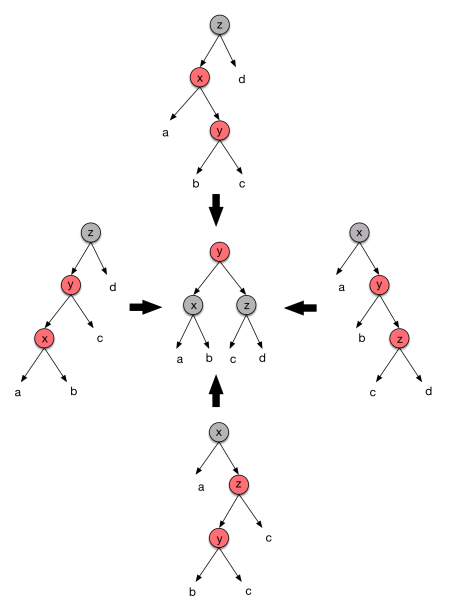
We assume that the subtrees a, b, c and d are balanced. For all these 4 cases we can perform a “rotation” to achieve the tree at the center.

The Black nodes constraint is not violated, because the path from the root still has the same number of Black nodes as before, and we fixed the consecutive Reds. Notice that y might violate the Red node constraints with its parent, so we need to do it recursively.

In terms of complexity, the insertion can be done in O(log n) and rebalancing takes a constant amount of time. Regarding the immutable structure, notice we only need to change nodes from the insertion path, so only O(log n) nodes have to be cloned.

My implementation for the Red Black tree in Ocaml is on github.

Conclusion

The first two chapters from this book are really interesting. I have seen the binomial heap and Red-Black trees before in data structure classes and also implemented some data structures such as AVL trees in functional programming in the past (Lisp) during college.

I wasn’t aware of the immutability of data in functional programming until much later, when I was learning Haskell. Okasaki first introduces this concept in Chapter 2, so it allow us keeping that in mind when studying the implementation of functional data structures.

He doesn’t make it explicit on Chapter 3 that the data structures presented are efficient in terms of extra memory necessary to clone them, but they are easy to see.

The ML syntax is very similar to OCaml, but it was a good exercise implementing the code on my own. I tried making it more readable with comments and longer variable names. This also led me to learn a few OCaml constructs and libraries, including:

• How to perform assertions (See the binomial heap implementation)
• Unit testing (using OUnit2 library)
• The “or matching” pattern (see the balance() function in red_black_tree.ml)

Source code | RSS feed | Tags: data structures ocaml