kuniga.me > NP-Incompleteness > Amortization Analysis

Amortization Analysis

21 Dec 2016

In Chapter 5 of Purely Functional Data Structures, Okasaki introduces the amortization analysis as preparation for the complexity analysis of functional data structures.

The idea of amortized analysis is to prove the complexity of an operation when the average cost per operation is less than the worst case cost of each individual operation.

In this post we’ll perform analysis of 2 data structures and show that their amortized running time is much better than their worst case. There are 2 methods presented in the book, the Banker’s Method and the Physicist Method. I found the Physicist easier to work with, so I’ll only use that. Also, I find it easy to understand concepts with an examples, so we’ll first introduce the data structure and then introduce the analysis.

Queue with lists

An easy way to implement the queue data structure is by using two lists, one representing the beginning (left) and the other the end (right). Inserting/removing an element from the beginning of a list in OCaml is O(1), while doing it at the end is O(n). For this reason, we store the end of the queue reversed in the right list. (In imperative languages the opposite is true, insertions/removals at the end are O(1) and at the beginning O(n), so the left array that is reversed).

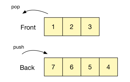
Insertions are performed by appending an element to the beginning of the right array. Removing from the front of the queue requires removing the first element of the left array. When the left array is empty, we need to reverse the contents of the right array and move it to the left.

We work with an invariant, in which the left array is only empty if the right array is empty as well. That requires a slight change to the removal, where we perform the reversal and move of the right array when the left array has only one element and is about to become empty.

I’ve implemented this idea in Ocaml.

Analysis - The Physicist Method

If we only look at the worst case, we will get that removing from a queue is an O(n) operation. We can improve this by looking at the amortized cost. One way to perform this analysis is via the physicist method, in which we define a potential (or cost) function \(\Phi(d)\) for the data structure \(d\). In the queue case, we can define it to be the size of the right list.

The amortized cost of step i, \(a_i\) is defined by

\[a_i = t_i + \Phi(d_i) - \Phi(d_{i-1})\]

Where \(t_i\) is the actual cost (in number of operations)

The intuition is that some costly operations such as reversing the list, which takes O(n) operations, can only happen after O(n) insertions happened, so the average cost per operation is O(1). Translating it to the potential analogy, each insersion operation increases the potential of the data structure by 1, so by the time a revert happens, the right list is emptied and that causes a loss of potential of n, which had been accumulated and that offsets the cost of the operation \(t_i\).

We can get the accumulated amortized cost of the operations up to a specific step by summing them, and we’ll get

\[A_i = T_i + \Phi(d_i) - \Phi(d_0)\]

If we choose \(\Phi(d)\) such that \(\Phi(d_i) \ge \Phi(d_0)\), for all i, then A_i is an upper bound of \(T_i\). Since we assume \(d_0\) is the empty queue, \(\Phi(d_0) = 0\) and we have \(\Phi(d_i) \ge 0\), this property is satisfied.

One important remark is that this analysis is only applicable to non-persistent data structures, which is not the case in OCaml. We present the OCaml code as exercise, but the correct analysis will done in later chapters.

Splay Trees

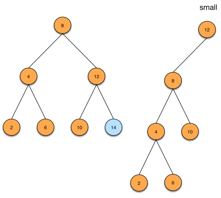
Splay Tree is a binary search tree. The insertion of an element e consists in spliting the current tree in 2 subtrees, one of all elements less or equal than e, which we’ll call small and another will all elements larger than e, which we’ll call big. We then make e the root of tree and small the left subtree and big the right subtree.

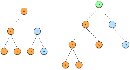
The partition operation is O(height of tree). The intuition is, when looking for the small subtree, imagine we’re analysing a node x. If x >= e, then we know all elements in the left subtree are also >= e, so are all the elements in the right subtree, so we can discard it and only look at the left subtree. The same idea applies to looking for the big subtree.

In an ideal scenario, the tree will be well balanced in such a way that the height of the tree is O(log n), and so the insertion operation. But that’s not always the case, so we introduce a balancing strategy. Whenever we follow 2 lefts in a row when searching for the big subtree, we perform a right rotation. Similarly, when following 2 rights in a row when searching for the small subtree, we perform a left rotation.

These re-balancing are enough to make partition and also insertion an O(log n) amortized time, as we shall see in the next section.

The operation for finding the minimum element is trivial. To delete the minimum element, we also perform rotations. Since we only traverse the left paths, we only have to do a left rotation.

I’ve implemented these ideas in OCaml.

Amortized Analysis of Splay Trees

We first define a potential function. Given a tree \(t\) and a node \(x \in t\), let \(t(x)\) be the subtree of \(t\) rooted in \(x\). Then \(\phi(t(x)) = \log(\mid t(x)\mid + 1)\) be a potential function where \(\mid t(x)\mid\) the number of nodes of the subtree of which \(x\) is root, and let the potential of a tree \(t\), \(\Phi(t)\), be the sum of the sub-potentials of all nodes of \(t\), that is,

(1) \(\Phi(t) = \sum_{x \in t} \phi(t(x))\).

The amortized equation of calling partition() is the actual cost of the partition, plus the potential of the resulting trees (small and big) minus the potential of the original tree. Let’s denote small(t) as \(s\), and big(t) as \(b\).

(2) \(\mathcal{A}(t) = \mathcal{T}(t) + \Phi(s) + \Phi(b) - \Phi(t)\)

We can prove that \(\mathcal{A}(t) \le 1 + 2 \log(\mid t \mid)\) (see appendix), which means the amortized cost of the partition operation is \(O(\log n)\). It implies that insertion also has an amortized cost of \(O(\log n)\).

The same idea can be used to prove the amortized costs of the deletion of the minimum element. Okasaki claims that splay trees are one of the fastest implementations for heaps when persistence is not needed.

Conclusion

I found amortized analysis very hard to grasp. My feeling is that the amortized analysis is too abstracted from the real problem, making it not very intuitive. It’s also not clear how one picks the potential function and whether there’s a choice of potential that might result in a better than the “actual” amortized cost.

Appendix

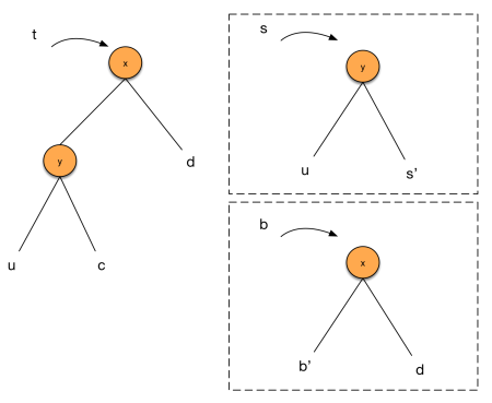
As we can see in code, there are four cases to consider: left-left, left-right, right-left and right-right. The left-* and right-* are symmetric, so let’s focus on the left-left and left-right cases. For the left-left case, suppose we perform the following partition:

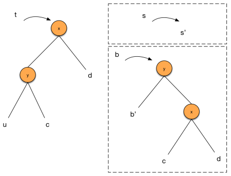
We start with (2)

(3) \(\mathcal{A}(t) = \mathcal{T}(t) + \Phi(s) + \Phi(b) - \Phi(t)\)

Since \(= \mathcal{T}\) corresponds to the number of recursive calls to partition, \(\mathcal{T}(t) = 1 + \mathcal{T}(u)\), so

(4) \(= 1 + \mathcal{T}(u) + \Phi(s) + \Phi(b) - \Phi(t)\)

The recursive call to u yields (s’, b’), so we have the equivalence, \(\mathcal{A}(u) = \mathcal{T}(u) + \Phi(s') + \Phi(b') - \Phi(u)\),

(5) \(= 1 + \mathcal{A}(u) - \Phi(s') - \Phi(b') + \Phi(u) + \Phi(s) + \Phi(b) - \Phi(t)\)

Since, s = s’,

(6) \(= 1 + \mathcal{A}(u) - \Phi(b') + \Phi(u) + \Phi(b) - \Phi(t)\)

and \(\Phi(b') - \Phi(b) = \phi(b(x)) + \phi(b(y)) + \Phi(c) + \Phi(d)\), and \(\Phi(t) - \Phi(u) = \phi(t(x)) + \phi(t(y)) + \Phi(c) + \Phi(d)\), we can cancel out some terms and simplify the equation above to

(7) \(= 1 + \mathcal{A}(u) - \phi(b(x)) + \phi(b(y)) - \phi(t(x)) - \phi(t(y))\)

by induction, \(\mathcal{A}(u) \le 1 + 2 \phi(u)\),

(8) \(\le 2 + 2\phi(u) + \phi(b(x)) + \phi(b(y)) - \phi(t(x)) - \phi(t(y))\)

Since \(u\) is a subtree of \(t(y)\), \(\phi(u) < \phi(t(y))\) and since the nodes in \(b\) is a subset of t, \(\phi(b(y)) \le \phi(t(x))\)

(9) \(< 2 + \phi(u) + \phi(b(x))\)

It’s possible to show that, given \(x, y, z\) such that \(y + z \le x\), then \(1 + \log y + \log z < 2 \log x\). We have that \(\mid t \mid = \mid u \mid + \mid c \mid + \mid d \mid + 2\), while \(\mid b(x)\mid = \mid c \mid + \mid d \mid + 1\), thus, \(\mid u \mid + \mid b(x)\mid < \mid t \mid\) and by the relation above, \(1 + \log (\mid u \mid) + \log (\mid b(x)\mid) + 1 < 2 \log (\mid t \mid) + 1\), \(\phi(u) + \phi(b(x)) + 1 < 2 \phi(t)\), which yields

(10) \(\mathcal{A}(t) < 1 + 2 \phi(t)\).

It’s very subtle, but in this last step we used the assumption of the rotation, in particular in \(\mid b(x)\mid = \mid c \mid + \mid d \mid + 1\), if we hadn’t performed the rotation, \(\mid b(x)\mid = \mid b \mid + \mid c \mid + \mid d \mid + 2\), and \(\mid u \mid + \mid b(x)\mid < \mid t \mid\) wouldn’t hold!

For the left-right case, we can do a similar analysis, except that now we’ll apply the recursion to \(c\), and the resulting partition will look different, as depicted below:

In this case, (8) will become

(11) \(\le 2 + 2\phi(c) + \phi(b(x)) + \phi(b(y)) - \phi(t(x)) - \phi(t(y))\)

We then use that \(\phi(c) < \phi(t(y))\) and \(\phi(t(y)) < \phi(t(x))\) this will allow us to cancel out some terms to

(12) \(< 2 + \phi(b(x)) + \phi(b(y))\)

Similar to what we've done before, we can show that \(\mid b(x)\mid + \mid b(y)\mid = \mid s \mid + \mid b \mid = \mid t \mid\) since the partitions of \(\mid t \mid\) are mutually exclusive. We can still use the result from the other case and get (10).

References

• [1] Wikipedia - Amortized Analysis