kuniga.me > NP-Incompleteness > The Gauss-Lucas Theorem
The Gauss-Lucas Theorem
03 Nov 2023
The Gauss-Lucas theorem (named after Carl Friedrich Gauss and Félix Lucas) describes a relationship between the roots of a polynomial and the roots of its derivarive when plotted in the complex plane. In particular it says that the roots of the derivative lie within the convex hull defined by the roots from the original polynomial or in less geometric terms, that each root of the derivative is a convex combination of the roots of the original polynomial.
In this post we’ll define the theorem more formally, present a proof and do some computational experimentation using Python.
Formal statement
Theorem. Let $P$ be a polynomial of degree $n$, of the form $P(x) = \sum_{k = 0}^n a_k z^k$, where $z, a_k \in \mathbb{C}$ and $a_n \neq 0$. Let $r_i$ be the zeros (or roots) of $P(z)$, that is $P(r_i) = 0$, for $i = 0, \dots, n$.
Consider its derivative $P’(z) = \sum_{k = 0}^{n-1} (k + 1) a_{k + 1} z^{k}$ and its corresponding roots $r’_j$ for which $P’(r’_j) = 0$, $j = 0, \dots, n - 1$.
Now, if we plot $r_i$ and $r’_j$ on the complex plane, the Lucas-Gauss theorem claims that $r’_j$ lies in the convex hull defined by $r_i$.
Experimentation
We can “visualize” this theorem by following these steps:
Step 1. (Generate) Generate N random complex numbers, $r$. Assume they’re the roots of a polynomial $P(z)$.
Step 2. (From roots) Compute the polynomial $P(z)$ from the roots $r$. We can do so using the fundamental theorem of algebra:
\[(2) \quad P(z) = \prod_{i = 1}^{n} (z - r_i)\]Step 3. (Derive) Compute the derivative of the polynomial, $P’(z)$, which is simply
\[P'(z) = \sum_{k = 0}^{n - 1} a_{k+1} (k + 1) x^{k}\]Where $a_{k}$ is the coefficient of $i$-th degree of $P(z)$.
Step 4. (Roots) Find the roots of $P’(z)$, $r’$. We can use one of the numeric algorithms to estimate the roots such as the Weierstrass method.
Step 5. (Convex Hull) Compute the convex hull of $r$ by assuming they’re 2D points. This can be done via some of convex hull algorithm such as Graham scan which runs in $O(n \log n)$.
Step 6. (Plot) Plot $r’$ and verify they lie inside the convex hull.
Python Implementation
Step 1. (Generate) We can generate the complex numbers using a uniform distribution and scale them to be a 10x10 square at the origin.
import random

N = 10
rs = []
for i in range(N):
    a = random.uniform(-5, 5)
    b = random.uniform(-5, 5)
    rs.append(a + b * 1j)
Note that Python supports complex numbers as first-class citizens! We can write a complex literal as:
c = 10 + 4j
c = 1j # imaginary only
It uses j instead of i and there’s no syntax for constructing the imaginary from a variable. However, the arithmetic operations work as one would expect, so if we want to construct a complex number with imaginary value from a real number stored in the variable x, we can do x * 1j.
Step 2. (From Roots) Numpy has a Polynomial class which we can use to perform all the operations we need in this experiment. It can be constructed from an array of coefficients c, where c[i] represents the coefficient of $i$-th degree.
The library also contains a utils function fromroots() which performs the product from $(2)$ and returns the coefficients which we can then use to construct the polynomial.
from numpy.polynomial.polynomial import Polynomial, polyfromroots
p0 = Polynomial(polyfromroots(rs))
Step 3. (Derive) The Polynomial class also supports computing its derivative via derive():
p1 = p0.deriv()Step 4. (Roots) The Polynomial class supports finding its roots via roots():
r1 = p1.roots()The documentation says the algorithm used for this is via enginevalues of the companion matrix. I have no idea how it works, but could be an interesting algorithm to explore in the future.
Step 5. (Convex Hull) We can using Scipy’s library for computing the 2D convex hull:
from scipy.spatial import ConvexHull

pts = [[r.real, r.imag] for r in rs]
hpts = [pts[idx] for idx in ConvexHull(pts).vertices]
From the documentation, this library implements the Quickhull algorithm.
Step 6. (Plot) For this step, we can use Matplotlib. We first plot r2 as a scatter plot:
import matplotlib.pyplot as plt

fig, ax =  plt.subplots(figsize=(18, 15))

xs = []
ys = []
for r in r2:
    xs.append(pts[0])
    ys.append(pts[1])
ax.scatter(xs, ys, color='#1f77b4')
And then draw a polygon corresponding to the convex hull vertices hpts:
import matplotlib.patches as patches
polygon = patches.Polygon(
    hpts,
    closed=True,
    edgecolor='black',
    facecolor='none'
)
ax.add_patch(polygon)
The full code is available as a Jupyter notebook on Github.
Results
Figure 1 contains the result for for N = 10. I experimented with larger number of points but noticed the root finding algorithm degrated a lot, by noticing that $\abs{P(r)} \gt 0$ for some roots found by the .roots() method.
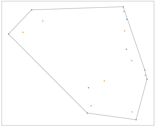
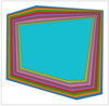
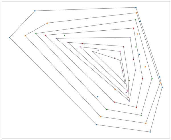
The image from the top of the post consists in applying this theorem recursively.
Conclusion
I learned about this theorem in the book Complex Analysis by Ahlfors, but the version presented there is a weaker one (in terms of half-planes) and it’s just called the Lucas Theorem. The theorem itself is relatively simple but it lends itself to a nice visualization, so I wanted to write a post about it.
The proof from this post is based on Wikipedia [1] but I found non-trivial to understand it, so I added a lot more steps and commentary.
