kuniga.me > NP-Incompleteness > The General Form of Cauchy's Theorem
The General Form of Cauchy's Theorem
15 Mar 2025
This is a post with my notes on complex integration, corresponding to Chapter 4 in Ahlfors’ Complex Analysis.
We previously studied the Cauchy Integral Theorem, which says that integrating a holomorphic function $f(z)$ over a closed curve results in 0. The results we obtained only applied if the domain of $f(z)$ is a circle or a rectangle.
In this post we want to generalize that result for other domains.
Chains and Cycles
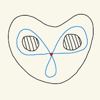
We define a chain as a “union” of arcs. For example in Figure 1. More formally we have:
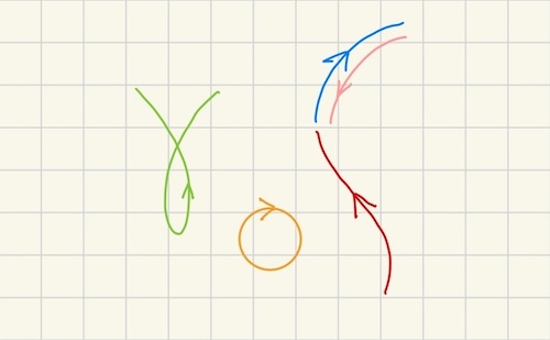
Definition. A chain is a set of arcs $\gamma_1, \gamma_2, \cdots, \gamma_n$, denoted by $\gamma_1 + \gamma_2 + \cdots + \gamma_n$ such that
\[\int_{\gamma_1 + \gamma_2} f(z)dz = \int_{\gamma_1} f(z)dz + \int_{\gamma_2} f(z)dz\]Noting that $\gamma_1, \gamma_2, \cdots, \gamma_n$ need not be connected. This notation is not particularly compact nor the definition illuminating, however the concept of equivalence of chains is useful.
Definition. We say that two chains $C_1$ and $C_2$ are equivalent if:
\[\int_{C_1} f(z)dz = \int_{C_2} f(z)dz\]for all functions $f$.
Here are some operations that preserve equivalence of chains:
- Permutating two arcs
- Subdividing an arc into multiple ones
- Merging multiple subarcs into one
- Removal of opposite arcs (i.e. cancelling them out)
In a chain can also have multiple copies of the same arc which we can denote via an appropriate coefficient, so a general form of a chain $\gamma$ is:
\[\gamma = \alpha_1 \gamma_1 + \alpha_2 \gamma_2 + \cdots + \alpha_n \gamma_n\]For non-negative (0 might be useful for ease of notation) integers $\alpha_i$ and distinct $\gamma_i$.
A cycle is analogous to a chain, except that the arcs must be closed curves.
Definition. A cycle is a chain in which all its arcs are closed curves.
Another way to define a cycle is as a chain in which each of its arcs have coinciding start and end points.
Simple Connectivity
A region is simply connected if it doesn’t have holes. More formally:
Definition. A region is simply connected if its complement with respect to the extended plane is connected.
Note the “with respect to the extended plane”. Which means the complement always includes the infinity. This is convenient to consider a parallel strip as simply connected, since a line partitions the unextended plane into two parts.
We can provide an alternative characterization of simple connectivity via winding numbers:
Theorem 1. A region $\Omega$ is simply connected if and only if $n(\gamma, a) = 0$ for all cycles $\gamma$ in $\Omega$ and all points $a$ not in $\Omega$.
First we prove that $H_1 \implies H_2$. This means that the complement of $\Omega$ is connected. Let $\gamma$ be a cycle in $\Omega$ and consider the regions defined by it. Let $\Gamma$ be the one containing $\infty$. Corollary 5 in [5] shows that $n(\gamma, a) = 0$ for $a \in \Gamma$. The complement of $\Omega$ is contained in $\Gamma$, so we arrive at statement $H_2$.
We now prove that $H_2 \implies H_1$ via count counter-positive ($\neg H_1 \implies \neg H_2$). This is almost obvious: if a region is not simply connected it contains a hole. There exists a cycle in $\Omega$ surrounding the hole and for any point $a$ in the hole we have $n(\gamma, a) = 1$ which implies $\neg H_2$ is true. But we need to provide a more precise way to find such cycle.
More formally, if the complement of $\Omega$ is not connected, it has multiple components one of them containing $\infty$. Let $A$ be one of the components not containing $\infty$ and $B$ the union of the other components. Let $\delta \gt 0$ be the shortest distance between a point in $A$ and $B$. We then tessalate the plane with a net of squares $Q$ with side $\lt \delta / 2$. Let $a$ be any point in $A$. We chose the tessalation so that $a$ lies in the center of a square. Notice by our choice of the square size, a given square cannot contain points from both $A$ and $B$.
Let $\partial Q$ be the curve corresponding to the boundary of the square $Q$ and oriented counter-clockwise. Consider the set indices $S$ of the squares that contain at least one point of $A$. We define the curve: $$\gamma = \sum_{j \in S} \partial Q_j$$ Because $A$ is a component, the internal sides of the squares cancel out and we're left with a curve that is a polygon with orthogonal sides.
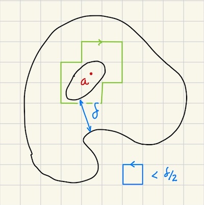
Since exactly one square in $S$ must contain $a$ by construct, we have that $n(\gamma, a) = 1$. As we claimed, a given square cannot contain points from both $A$ and $B$, so no square in $S$ intersects $B$, and so does $\gamma$.
We also claim that no point in $\gamma$ belongs to $A$: if it did, it would have to exist on the boundary of at least two squares and they would have cancelled out. This means that $\gamma$ is contained enriely within $\Omega$.
Homology
Definition. A cycle $\gamma$ in an open set $\Omega$ is homologous to zero with respect to $\Omega$, denoted by $\gamma \sim 0 \, (\mbox{mod } \Omega)$, if $n(\gamma, a) = 0$ for all points $a$ in the complement of $\Omega$.
We can simply say $\gamma \sim 0$ if the open set $\Omega$ is implied from context. We can also define the notation $\gamma_1 \sim \gamma_2$ to mean $\gamma_1 - \gamma_2 \sim 0$.
Note that if $\Omega$ is a simply connected region, by Theorem 1 all cycles in it are homologous to zero. In this sense homology is a more general property of cycles, which will allow us to extend some results to non-simply connected regions.
Cauchy Integral Theorem
We’re ready to state the first generalization of Cauchy Integral Theorem:
Theorem 2. If $f(z)$ is holomorphic in $\Omega$, then
\[(1) \quad \int_\gamma f(z) dz = 0\]For any cycle $\gamma$ satisfying $\gamma \sim 0 \, (\mbox{mod } \Omega)$.
Notice that in this result we don’t assume anything about $\Omega$. However, if it’s a simply connected region, then all cycles in it are homologous to zero, so we can claim that:
Corollary 3. If $f(z)$ is holomorphic in a simply connected region $\Omega$, then
\[\int_\gamma f(z) dz = 0\]For any cycles in $\Omega$.
So until now, we knew that $(1)$ held as long as $\Omega$ as a circle or rectangle, but now we have relaxed the condition to any simply connected region!
This also means we can generalize Cauchy’s Integral Formula [6] to simply connected regions.
This is the main result we wanted to prove in this post. We now consider some variants and further generalizations.
Locally Exact Differential
In our post Path-Independent Line Integrals [3], we said that a line integral $\int_\gamma f(z)dz$ can be expressed as a function of its real and imaginary parts: $\int_\gamma p(x)dx + q(y)dy$ or $\int_\gamma pdx + qdy$ for short. This form of the integrand is defined as a differential form. In this case, we can call its integrand a differential.
The differential $p dx + q dy$ is called an exact differential in $\Omega$ if there exists a function $U(x, y): \Omega \rightarrow \mathbb{R}$ such that $\partial U(x, y)/\partial x = p(x)$ and $\partial U(x, y)/\partial y = q(y)$ or more concisely, that $dU = pdx + qdy$ [3].
Definition. A differential $p dx + q dy$ is called a locally exact differential if it’s exact in some neighborhood of every point in the domain $\Omega$.
More precisely, suppose $p dx + q dy$ is a locally exact differential. Then for each $a \in \Omega$, there must exist a neighborhood $N(a)$ such that there exists $U(x, y)$ with $dU = pdx + qdy$ for each $(x, y)$ in $N(a)$.
Note that a exact differential is a more strict condition than a locally exact differential. In an exact differential the existence of $U(x, y)$ with $dU = pdx + qdy$ must hold for all points in its domain. Thus a exact differential implies locally exact differential.
We’ve seen in Theorem 1 in [3] that the exact differential $\int_\gamma p dx + q dy$ only depends on the endpoints of $\gamma$. This means that if $\gamma$ is a closed curve, we can split it into $\gamma = \gamma_1 + \gamma_2$ where $\gamma_1$ and $\gamma_2$ share endpoints. Thus we have that $\int_{\gamma_1} p dx + q dy = -\int_{\gamma_2} p dx + q dy$ implying that $\int_\gamma p dx + q dy = 0$. In other words, exact differentials satisfies $(1)$ without any specific constraints on the domain, $f$ also doesn’t need to be holomorphic.
We can obtain an analogous result for locally exact differentials:
Theorem 4. $p dx + q dy$ is a locally exact differential in $\Omega$, then
\[\int_{\partial \gamma} p dx + q dy = 0\]For every cycle $\gamma \sim 0$ in $\Omega$.
So in [3] we showed that an exact integral satisfied $(1)$ if $\gamma$ happens to be a Jordan curve. Now we relaxed the condition for locally exact integrals and $\gamma$ to cycles homologous to $0$ (which are more general than Jordan curves).
Multiply Connected Regions
Now we consider regions with holes. The idea is to decompose the problem and express the integral a linear combination of one integral per hole.
A region that is not simply connected is multiply connected, in other words, it contains holes. Here we restrict ourselves to finite connectivity, where the number of holes is finite.
A precise definition of finite connectivity is that the complement of a region $\Omega$ with respect to the extend plane are $n$ components $A_1, \cdots, A_n$, where by convention the $A_n$ region is the “external” to $\Omega$, the one containing $\infty$.
Consider a cycle $\gamma$ in $\Omega$. As we proved in [5], points within the same component $A_i$ have the same winding number with respect to $\gamma$. Intuitively, since $\gamma$ cannot cut throught $A_i$, it must wind around it and thus around its points the same amount of times. We can thus associate a winding number to each of the components $A_i$, and call them $c_i$.
We can then decompose the cycle into multiple closed curves, such that it winds around a component at most once. See Figure for an example. If a closed curve $\delta$ does not wind around any regions, then we have $n(\delta, a) = 0$ for all points in the complement of $\Omega$ and thus $\delta \sim 0$.
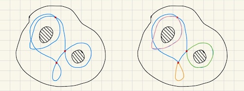
If $\delta$ does wind around a region $A_i$, it does so exactly once, because otherwise it would self-intersect and we would have split into multiple curves. We can choose a “canonical” close curve for each $A_i$ which we call $\gamma_i$ which winds around it exactly once. Let $a$ be a point in $A_i$, we then have $n(\delta, a) = n(\gamma_i, a)$ or that $\delta - \gamma_i \sim 0$.
So for each closed curve in the original $\gamma$, we can find a corresponding $\gamma_i$ to “neutralize” it, so we arrive at:
\[\gamma - \sum_{i = 1}^{n-1} c_i \gamma_i \sim 0\]Note that we don’t have $\gamma_n$ because that’s the “external” region. Apply Theorem 2 to this curve:
\[\int_{\gamma - \sum_{i = 1}^{n-1} c_i \gamma_i} f(z)dz = 0\]Splitting into separate integrals (from the definition of chains):
\[\int_{\gamma} f(z)dz - \sum_{i = 1}^{n-1} c_i \left(\int_{\gamma_i} f(z)dz \right) = 0\]or that
\[\int_{\gamma} f(z)dz = \sum_{i = 1}^{n-1} c_i \left(\int_{\gamma_i} f(z)dz \right)\]This allows us compute the integral over a complex curve from a linear combination of the integrals over simpler curves. Let’s define
\[P_i = \int_{\gamma_i} f(z)dz\]as the module of periodicity of $f dz$. We note that $\gamma_i$ is dependent only on $\Omega$ (more specifically the region $A_i$ of its complement) and not on the curve $\gamma$ and thus $P_i$ is only dependent on $f$ and $\Omega$.
Example
Let’s look at an example of the application of the result above. Consider the region $\Omega$ defined as
\[r_1 \lt \abs{z} \lt r_2\]that is, an annulus. The complement of this region is $A_1: \abs{z} \le r_1$ and $A_2: \abs{z} \ge r_2$. A possible canonical closed curve winding around $A_1$ is $C: \abs{z} = r_1 + \epsilon$ for some $\epsilon \gt 0$.
From our results above, we have
\[\int_{\gamma} f(z)dz = c_1 \int_C f(z) dz\]Where $c_1$ is the number of times a given cycle $\gamma$ winds around $A_1$.
Conclusion
In this post we learned about a generalization of the Cauchy Integral Theorem for other domains, in particular simply connected regions.
We went a step further and generalized the theorem for the so called curves that are homologous to 0. We also generalized the results from path independent integrals [3] for these type of curves.
We finally considered multiply connected regions (those with holes) and found a way to make any cycle homologous to zero via modules of periodicity and that allowed us to apply the general form of the Cauchy Integral Theorem. This in turn led to a formula for computing the integral of $f(z)$ over an arbitrary cycle as a linear combination of the modules of periodicity of $f(z)$.
The modules of periodicity will be useful in our next top of study, The Calculus of Residues.
