kuniga.me > NP-Incompleteness > Zeros and Poles
Zeros and Poles
02 Nov 2024
This is the 8-th post in the series with my notes on complex integration, corresponding to Chapter 4 in Ahlfors’ Complex Analysis.
In this post we’ll cover poles, a special type of isolated singularity, in the context of holomorphic functions.
The previous posts from the series:
- Complex Integration
- Path-Independent Line Integrals
- Cauchy Integral Theorem
- The Winding Number
- Cauchy’s Integral Formula
- Holomorphic Functions are Analytic
- Removable Singularities
In the last post we talked about removable singularities. We learned that it’s a special case of what is called isolated singularities. In this post we’ll talk about another type of isolated singularity, known as a pole, and its counterpart, a zero.
Removable singularities are “nice” because we’ve learned that we can extend holomorphic functions to remove it. The constraint is that the singularity $a$ must satisfy $\lim_{z \rightarrow a} (z - a) f(z) = 0$.
As Corollary 6. in [3] shows, this also implies that $\lim_{z \rightarrow a} f(z)$ exists (it’s finite). In this post we’ll consider the case in which $\lim_{z \rightarrow a} f(z) = \infty$. If we 3D-plot the magnitude of a complex function $f$ (where $xy$-plane is the complex and $z$-axis is the magnitude) we’ll obtain a surface that looks like a pole of sorts around $a$.
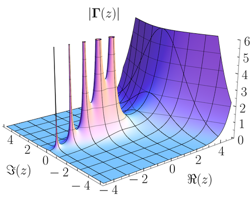
Hence the name of this singularity is simply known as pole.
Definition
Let $f$ be a holomorphic function in $\Omega \setminus a$. A point $a$ is a zero of $f$ if $f(a) = 0$. Conversely, a point $a$ is a pole of $f$ if it’s a zero of $1/f$, i.e. $1/f(a) = 0$.
More generally, a point $a$ is a zero of order $m$ if $a$ is a zero for all the $n$-th derivatives of $f$ for $n = 1, \cdots, m - 1$, but not for $m$. Similarly, a point $a$ is a pole of order $m$ if it’s a zero of order $m$ of $1/f$.
In order to provide different characterizations of zeros and poles, we shall introduce Laurent Series. Before we do so, we need to define Annular regions.
Annular Region
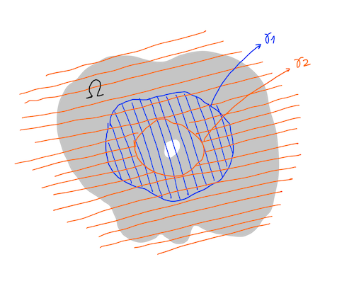
Let $\gamma_1$ and $\gamma_2$ be two simple closed counter-clockwise curves in $\Omega$, where $\gamma_2$ is contained inside $\gamma_1$. Denote by $\mbox{int}(\gamma)$ the set of points in the interior of the closed curve $\gamma$ (which excludes points on the curve) and $\mbox{ext}(\gamma)$ the set of points in the exterior of $\gamma$ (also excludes points on the curve).
We define the annular region of $\gamma_1$ and $\gamma_2$ as $\mbox{ext}(\gamma_2) \cap \mbox{int}(\gamma_1)$, that is the set points that are contained inside $\gamma_1$ but outside $\gamma_2$. We’ll denote this set by $\circledcirc(\gamma_1, \gamma_2)$, but we’ll omit the arguments when the curves involved are implied.
If we assume the curves are concentric circles and we draw this region in the plane it will look like a ring, which is annulus in Latin, and hence the name annular region.
Lemma 1. (Cauchy Integral Formula decomposition in annular regions). Let $f: \Omega \rightarrow \mathbb{C}$ be a holomorphic function and $\gamma_1$ and $\gamma_2$ be two simple closed counter-clockwise curves in $\Omega$, where $\gamma_2$ is contained inside $\gamma_1$ and $\gamma_1$ inside $\Omega$. Then there exists holomorphic functions $f_1: \Omega \cup \mbox{int}(\gamma_1) \rightarrow \mathbb{C}$ and $f_2: \Omega \cup \mbox{ext}(\gamma_2) \rightarrow \mathbb{C}$ such that:
\[(1) \quad f(z) = f_1(z) + f_2(z)\]for $z \in \Omega$, with
\[\lim_{z \rightarrow \infty} f_2(z) = 0\]This decomposition is unique and we can write:
\[(2) \quad f_1(z) = \frac{1}{2\pi i} \int_{\gamma_1} \frac{f(w)}{w - z}dw\]for $z \in \mbox{int}(\gamma_1)$, and:
\[(3) \quad f_2(z) = -\frac{1}{2\pi i} \int_{\gamma_2} \frac{f(w)}{w - z}dw\]for $z \in \mbox{ext}(\gamma_2)$ and:
\[(4) \quad f(z) = \frac{1}{2\pi i} \int_{\gamma_1} \frac{f(w)}{w - z}dw -\frac{1}{2\pi i} \int_{\gamma_2} \frac{f(w)}{w - z}dw\]for $z \in \circledcirc(\gamma_1, \gamma_2)$.
Part 1: Uniqueness. First we show that the decomposition is unique. Suppose $f$ can be decomposed in such a way into $f_1, f_2$ and $g_1, g_2$, with $f = f_1 + f_2 = g_1 + g_2$. Then $f_1 - g_1$ is holomorphic in $\Omega_1$ and $g_2 - f_2$ is holomorphic in $\Omega_2$. In the shared domain $\Omega = \Omega_1 \cap \Omega_2$, we have that $f_1 - g_1 = g_2 - f_2$.
So we can define a function $F: \mathbb{C} \rightarrow \mathbb{C}$ which equals to $f_1 - g_1$ in $\Omega_1 \setminus \Omega$, equals to $g_2 - f_2$ in $\Omega_2 \setminus \Omega$ and equals to either in $\Omega$. These sets partition the complex plane, so $F$ is holomorphic in the entirety of $\mathbb{C}$.
Since $F(z) = g_2(z) - f_2(z)$ as $z$ goes to infinity (because $\Omega_2$ includes the exterior of $\gamma_1$), and we know that $\lim_{z \rightarrow \infty} f_2(z) = \lim_{z \rightarrow \infty} g_2(z) = 0$ by definition, so $\lim_{z \rightarrow \infty} F(z) = 0$. This means $F$ is bounded in the whole plane, and by Liouville's Theorem (Theorem 7 in [6]), we conclude that $F(z) = 0$ on the whole plane, proving that $f_1 = g_1$ and $f_2 = g_2$.
Part 2. We now wish to prove that $f(z)$ can be written as $(4)$ for $z \in \circledcirc(\gamma_1, \gamma_2)$. For any such $z$, we have the winding number [7] $n(\gamma_1, z) = 1$ because $z$ is contained inside $\gamma_1$ and it's a counter-clockwise curve. We have $n(\gamma_2, z) = 0$ because $z$ is always outside of $\gamma_2$.
Recall that the definition of a winding number for an arbitrary closed curve $\gamma$ is [6]: $$ n(\gamma, z) = \frac{1}{2\pi i} \int_{\gamma} \frac{dw}{w - z} $$ Adding $n(\gamma_1, z)$ and $n(\gamma_2, z)$ and multiplying by $f(z)$ gives us: $$f(z) = \frac{1}{2\pi i} \int_{\gamma_1} \frac{f(z) dw}{w - z} - \frac{1}{2\pi i} \int_{\gamma} \frac{f(z) dw}{w - z}$$ Subtracting it from $(4)$: $$0 = \frac{1}{2\pi i} \int_{\gamma_1} \frac{f(w) - f(z)}{w - z}dw - \frac{1}{2\pi i} \int_{\gamma_2} \frac{f(w) - f(z)}{w - z}dw$$ So to show that $f$ can be written as $(4)$, we can prove that: $$ \int_{\gamma_1} \frac{f(w) - f(z)}{w - z}dw = \int_{\gamma_2} \frac{f(w) - f(z)}{w - z}dw $$ Let $f'(w) = f(w) - f(z)$. Because $f'(w)$ is analytic and $f'(z) = 0$, by the Factor theorem for analytic functions [8], there exists another analytic function $F(w)$ such that $f'(w) = F(w) (w - z)$, so we reduce the problem to proving: $$ \int_{\gamma_1} F(w)dw = \int_{\gamma_2} F(w)dw $$ Let $z_1$ be a point in $\gamma_1$ and $z_2$ be a point in $\gamma_2$. We connect them by a path $\gamma_3$ and another slighly parallel path $\gamma_4$ such that they're not more than a $\epsilon$ apart (see Figure 1.1).
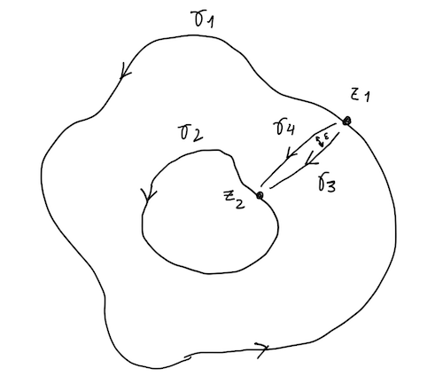
The path formed via $\gamma_1 \rightarrow \gamma_3 \rightarrow (-\gamma_2) \rightarrow (-\gamma_4)$ forms a closed curve contained in $\Omega$. Let's define it as $\gamma_\epsilon$ where $\epsilon$ determines how close $\gamma_3$ and $\gamma_4$ are. Thus, for any holomorphic function in $\Omega$, including $F(w)$ defined above, Cauchy's Integral Theorem [9] says: $$\int_{\gamma_\epsilon} F(w)dw = 0$$ If $\epsilon \rightarrow 0$, then $\gamma_3 \rightarrow \gamma_4$, amd this becomes: $$\int_{\gamma_1} F(w)dw - \int_{\gamma_2} F(w)dw = 0$$ Which demonstrates $f(z)$ can be written as $(4)$.
Part 3. It remains to show that $f$ can be written as $f_1 + f_2$, defined as in $(2)$ and $(3)$. We define $f_1(z)$ as: $$ \begin{equation} f_1(z)=\left\{ \begin{array}{@{}ll@{}} \frac{1}{2\pi i} \int_{\gamma_1} \frac{f(w)}{w - z}dw, & \text{if}\ z \in \mbox{int}(\gamma_1) \\ f(z) + \frac{1}{2\pi i} \int_{\gamma_2} \frac{f(w)}{w - z}dw, & \text{if}\ z \in \Omega \cap \mbox{ext}(\gamma_2) \end{array}\right. \end{equation} $$ Note that $\mbox{int}(\gamma_1)$ and $\Omega \cap \mbox{ext}(\gamma_2)$ are not disjoint. In fact their intersection is exactly the annular region, for which we must have: $$\frac{1}{2\pi i} \int_{\gamma_1} \frac{f(w)}{w - z}dw = f(z) + \frac{1}{2\pi i} \int_{\gamma_2} \frac{f(w)}{w - z}dw$$ Which is consistent with $(4)$. With Lemma 6 (*Appendix*) we can prove that $f_1$ is holomorphic for both $\mbox{int}(\gamma_1)$ and $\Omega \cap \mbox{ext}(\gamma_2)$, and hence it should be holomorphic in $\Omega_1$. It's hard for me to "see" that because $f_1$ has different definitions and seems to have a point of discontinuity somewhere in its domain which would make it non-holomorphic.
Similarly, for $f_2(z)$: $$ \begin{equation} f_2(z)=\left\{ \begin{array}{@{}ll@{}} - \frac{1}{2\pi i} \int_{\gamma_2} \frac{f(w)}{w - z}dw, & \text{if}\ z \in \mbox{ext}(\gamma_2) \\ f(z) - \frac{1}{2\pi i} \int_{\gamma_1} \frac{f(w)}{w - z}dw, & \text{if}\ z \in \Omega \cap \mbox{int}(\gamma_1) \end{array}\right. \end{equation} $$ Again, $\mbox{ext}(\gamma_2)$ and $z \in \Omega \cap \mbox{int}(\gamma_1)$ are not disjoint, and their intersection is their annular region, where we have: $$-\frac{1}{2\pi i} \int_{\gamma_2} \frac{f(w)}{w - z}dw = f(z) - \frac{1}{2\pi i} \int_{\gamma_2} \frac{f(w)}{w - z}dw$$ which is also consistent with $(4)$. We can use Lemma 6 again to show that $f_2$ is holomorphic in $\Omega_2$.
The result makes intuitive sense in light of the original Cauchy Integral Formula. If we assume the annular region has no holes, then $\gamma_2$ vanishes, and $f(z)$ coincides with $f_1(z)$ which is the same the original Cauchy Integral Formula.
Where there’s a hole, we need to subtract that portion ($f_2(z)$) from $f_1(z)$, which is what $(4)$ does.
Laurent Series
Let’s consider the special annular region $\curly{z \mid r \lt \abs{z - a}\lt R} \in \Omega$ for $0 \le r \le R \le \infty$, that is, the region where $\gamma_1$ is the circle of radius $R$ and $\gamma_2$ the circle of radius $r$. Assume that $a \not \in \Omega$.
Let $f$ be a holomorphic function in $\Omega$. From Lemma 1 we know there are functions $f_1: \Omega \cup \mbox{int}(\gamma_1)$ and $f_2: \Omega \cup \mbox{ext}(\gamma_2)$ such that $f = f_1 + f_2$.
Let $D$ be the open disk of radius $R$ centered in $a$. Note that $D$ is not contained in $\Omega$ due to its center $a$, but it is contained in $\Omega \cup \mbox{int}(\gamma_1)$. So $f_1$ is holomorphic in $D$ and thus analytic and the series
\[(5) \quad f_1(z) = \sum_{n = 0}^{\infty} c^{(1)}_n (z - a)^n\]converges for $z \lt R$. Unfortunately $D$ is not contained in $f_2$’s domain, $\Omega \cup \mbox{ext}(\gamma_2) = D \setminus \curly{a}$. However, we can still express $f_2$ as a convergent series:
Lemma 2. Let $f_2$ be a holomorphic function in $\Omega \cup \curly{z : \abs{z - a} \gt r}$, where $a \not \in \Omega$. Then it can be written as a series:
\[(6) \quad f_2(z) = \sum_{n = -\infty}^{0} c^{(2)}_n (z - a)^n\]Tha converges for $\abs{z - a} \gt r$.
Let's find out the domain of $f'_2$, by transforming the domain $f_2$, $D \setminus \curly{a}$ using $t$. Subtracting $a$ corresponds to moving $D$ to be centered at the origin. Then we perform a inversion. We've seen in [5] that inverting a circle of radius $R$ and center $z_0$ with $R \ne \abs{z_0}$ (true in this case) gives as a circle of radius $$R' = \left\lvert \frac{R}{R^2 - \abs{z_0}^2} \right\rvert$$ Which in this case is $1/R$. So the domain of $f'_2$ is the disk $D'$ of radius $1/R$ minus the origin.
Since $t$ is a Möbius transformation, it's a holomorphic function for $z \ne a$. So it's inverse is also a Möbius transformation, and since the composition of functions preserve holomorphism, $f'_2$ is holomorphic.
When $z \rightarrow 0$ in this domain, it goes to $\infty$ and by Lemma 1, $\lim_{z \rightarrow \infty} f_2(z) = 0$, so $\lim_{z \rightarrow 0} f'_2(0) = 0$. Thus $0$ is a removable singularity of $f'_2$, and we can find a holomorphic function $g'_2$ and thus analytic over the disk $D'$ and it has a convergent series representation: $$g'_2(z) = \sum_{n = 0}^{\infty} c'_n z^n$$ We can apply $t(z)$ over this series to obtain: $$f_2(z) = (g'_2 \circ t)(z) = \sum_{n = 0}^{\infty} c'_n \left(\frac{1}{z - a}\right)^n$$ For $z \in D \setminus \curly{a}$. If we re-index $n$ so it goes from $-\infty$ to $0$ and re-labeling $c'_n$, we get: $$f_2(z) = \sum_{n = -\infty}^{0} c^{(2)}_n (z - a)^n$$ QED.
Replacing $(5)$ and $(6)$ in $(1)$ gives us:
\[(7) \quad f(z) = \sum_{n = -\infty}^{\infty} c_n (z - a)^n\]For $z$ in $\curly{z : r \lt \abs{z - a}\lt R} \in \Omega$. Where $c_n = c^{(2)}_n$ for $n < 0$, $c_n = c^{(1)}_n$ for $n > 0$ and $c_0 = c^{(1)}_0 + c^{(2)}_0$. This is defined as the Laurent Series.
Now suppose $\Omega$ contains a single singularity $a$. We can have the annulus centered in $a$ and make $r$ arbitrarily small and $R$ arbitrarily large so that is almost coincides with $\Omega$.
Thus we can think of $(4)$ as generalizing Cauchy Integral Formula for a region with holes and $(7)$ as generalizing analytic functions for a region with holes.
The Laurent series are named after Pierre Alphonse Laurent, who wrote about them in 1843. Karl Weierstrass had previously described it in a paper written in 1841 but it was only published in 1894.
Isolated Singularities
The Laurent series provide a very simple way to distinguish between classes of isolated singularities.
Removable Singularities
Lemma 3. Let $f$ have Laurent series as in $(7)$. Then, if $c_n = 0$ for all $n < 0$ then $a$ is a removable singularity.
So $g$ is a holomorphic extension of $f$, with $f(z) = g(z)$ for $z \ne a$ and $\lim_{z \rightarrow a} f(z) = g(a)$.
A special case is if $c_n = 0$ for all $n < m$, for $m \ge 1$ (i.e. the $m$ first coefficients of the Taylor series are also 0). Then $f(z)$ has a zero of order $m$. We can conclude that $a$ is such zero from the Taylor series.
Note that if $f(z)$ has $a$ as its zero of order $m$, it can be written as
\[f(z) = (z - a)^m f_m(z)\]Where $f_m(z)$ has a valid Taylor series representation and is thus holomorphic.
Poles
Lemma 4. Let $f$ have Laurent Series as in $(7)$. Then, if $c_n = 0$ for all $n < -m$ and $c_{-m} \ne 0$ for some finite $m > 0$, $a$ is a pole of order $m$ of $f$.
First we define $g(z) = (z - a)^m f(z)$, which gets rid of the terms with $(z - a)$ in the denominator in the Laurent series, making $g(z)$ holomorphic (even at $a$) with the a Taylor series : $$g(z) = \sum_{n = 0}^{\infty} c_{n - m} (z - a)^n$$ Where the coefficients are the same as in $(7)$. Since $g(a) = c_{-m}$, and by hypothesis $c_{-m} \ne 0$, we have $g(a) \ne 0$. Let's consider the inverse of $f$, $h(z) = 1/f(z)$. We have: $$h(z) = \frac{1}{f(z)} = \frac{(z - a)^m}{g(z)}$$ Let's define $h_m(z) = 1/g(z)$ so: $$h(z) = (z - a)^m h_m(z)$$ The function $h_m$ is holomorphic everywhere, even at $a$ because $g(a) \ne 0$, which means we can write $h_m(z)$ as a the Taylor series: $$h_m(z) = \sum_{n = 0}^{\infty} c'_n (z - a)^n$$ We can obtain $h(z)$'s Taylor series by multipling the terms above by $(z - a)^m$: $$h(z) = \sum_{n = 0}^{\infty} c'_n (z - a)^{n + m}$$ Note the coefficients $c'_n$ are the ones from $h_m(z)$'s Taylor series. It's clear that the first $m - 1$ derivatives of $h(z)$ contain the term $(z - a)$ and is thus 0 for $z = a$. For the $m$-th derivative we'd have: $$h^{(m)}(z) = \sum_{n = 0}^{\infty} c'_n (z - a)^{n} \prod_{p = n + 1}^{n + m} p$$ For $h^{(m)}(a)$ we get $c'_0 \prod_{p = 1}^{m} p$. Now since $g(a) \ne 0$, then $h_m(a) \ne 0$ and hence $c'_0 \ne 0$ and finally $h^{(m)}(a) \ne 0$. In other words, $h(z)$, $1/f(z)$, has a zero of order $m$. Thus we conclude that $f(z)$ has a pole of order $m$.
Essential Singularities
Another way to word the hypothesis of Lemma 4 is to that the Laurent series contains a finite number of non-zero “negative” coefficients. If it has an infinite number, then we have what is called an essential singularity, which is by definition any isolated singularity that is neither removable nor a pole.
Essential singularies are weird. The Casorati-Weierstrass theorem highlights this by saying that if $a$ is an essential singularity of $f(z)$, then $f$ comes arbitrarily close to any complex number near $a$. For formally:
Theorem (Casorati-Weierstrass) If $a$ is an essential singularity of $f(z)$, then every point $c \in \mathbb{C} \cup \curly{\infty}$ is a limit point of $f(z)$ as $z \rightarrow a$.
Let's start by proving through contrapositive the special case $c = \infty$. We assume $\infty$ is not a limit point of $f(z)$. Then $\lim_{z \rightarrow a} f(z)$ is finite and by Corollary 6 in [3], it implies that $a$ is a removable singularity, which is not an essential singularity by definition.
Now suppose $c \ne \infty$. We again prove through contrapositive, by assuming $c$ is not a limit point of $f(z)$. In particular for $z \in \Omega \setminus \curly{a}$, $f(z)$ is holomorphic and it doesn't intersect the neighborhood of $c$, $\abs{z - c} \lt \epsilon$. Let's define $$g(z) = \frac{1}{f(z) - c}$$ For the domain $\Omega \setminus \curly{a}$ is holomorphic because $f(z)$ is holomorphic and $f(z) \ne c$. In particular this function is bounded by $1/\epsilon$. Since $\lim_{z \rightarrow a} g(z)$ is finite, by Corollary 6 in [3], we conclude that $a$ is a removable singularity and thus $g(z)$ can be extended to be holomorphic in $\Omega$. This means we can assume that $g(a)$ exists. We can then write $f$ in term of $g$: $$f(z) = \frac{1}{g(z)} + c$$ and that $$\frac{1}{f(z)} = \frac{g(z)}{1 + c g(z)}$$ If $g(a)$ is 0, then $1/f(z)$ is also 0, so $a$ is a zero of $1/f$ and by definition a pole of $f(z)$. If $g(a)$ is non-zero, then $f(a)$ is defined and $a$ is a removable singularity of $f(z)$. In either case, $a$ is not an essential singularity of $f(z)$ as we wished to show. QED.
More Definitions
Now that we have defined Laurent series and the three different types of isolated singularities, we can introduce some other useful terminology.
Singular and Analytic Parts
A function can be decomposed into two, based on its Laurent series. The series containing the terms for $n \lt 0$ are called the singular part of $f(z)$ and those for $n \ge 0$ are the analytic part.
For analytic functions (which are holomorphic) the singular part is 0. Conversely, if its singular part is non-zero, we know it contains a singularity. This terminology makes sense!
Meromorphic Functions
Functions whose isolated singularity form a pole are called meromorphic functions. This comes from the Greek meros, part, in contrast with holos, meaning whole. Some definitions of meromorphic functions include functions with removable singularities, but as we’ve learned these functions are holomorphic functions in disguise.
The term was coined by Karl Weierstrass.
Conclusion
In this post we explored a type of isolated singularity that’s more problematic than a removable singularity: a pole.
As part of the process, we also learned about Laurent series which is a generalization of the Taylor series and the generalization of the Cauchy Integral Formula for annular regions. With these, we’re able to distinguish between the three types of isolated singularities, removable singularities, poles and essential singularities.
Essential singularities are the most problematic of the three. I was initially thinking of dedicating an entire post for it, but it seems like there not as many interesting results about it, except the Casorati-Weierstrass theorem which we included here.
The book from Ahlfors [1] is particularly difficult to follow on this topic. I had to complement it a lot with Tao’s notes [4], much like I had to do with the previous post on this topic [3].
Appendix
Lemma 5. Let $f(z, t): \Omega \times [0, 1] \rightarrow \mathbb{C}$ be a continuous function such that for a given $t$, $g_t(z) = f(z, t)$ is holomorphic. Then
\[(8) \quad F(z) = \int_{0}^{1} f(z, t) dt\]is also holomorphic.
Note: Lemma is listed as Exercise 38 in Tao's blog [8], without an answer. I found the proof in Stein and Shakarchi's book [10].
Lemma 6. Let $f(z)$ be a holomorphic function in a region $\Omega$. Let $\gamma$ be a curve contained in $\Omega$. Then
\[g(z) = \int_{\gamma} \frac{f(w)}{w - z}dw\]is holomorphic, for $z$ not in $\gamma$.
We can also parametrize the curve, so that $w = \gamma(t)$ for $0 \le t \le 1$. This lets us rewrite $g(z)$ as: $$ g(z) = \int_0^1 \frac{f(\gamma(t))}{\gamma(t) - z} \gamma'(t)dt $$ Let's define $$ h(z, t) = \frac{f(\gamma(t))}{\gamma(t) - z} \gamma'(t) $$ For a fixed $t$, we have that $\gamma(t)$ is a point inside $\Omega$ and hence $f(\gamma(t))$ is holomorphic, and $\gamma'(t)$ is a constant. Since $z$ is not in $\gamma$, the denominator is non-zero and thus $h(z, t)$ is holomorphic. We can use Lemma 5 to conclude that $g(z)$ is also holomorphic.
References
- [1] Complex Analysis - Lars V. Ahlfors
- [2] Wikipedia: Zeroes and Poles
- [3] NP-Incompleteness: Removable Singularities
- [4] What’s new - Math 246A, Notes 4: singularities of holomorphic functions
- [5] NP-Incompleteness: Möbius Transformation
- [6] NP-Incompleteness: Cauch integral formula
- [7] NP-Incompleteness: The Winding Number
- [8] What’s new - Math 246A, Notes 3: Cauchy’s theorem and its consequences
- [9] NP-Incompleteness: Cauchy Integral Theorem
- [10] Complex Analysis - Stein and Shakarchi
