kuniga.me > NP-Incompleteness > Topological Equivalence
Topological Equivalence
03 Nov 2022
I’ve recently read the book Introduction to Topology by Bert Mendelson [1] and before that my only knowledge of topology is that some objects are topologically equivalent, for example a mug and a doughnut.
After reading the book, I found topology is a lot more about algebraic formalism than visual geometry. So in this post I’d like to discuss the idea of topological equivalence from this formal perspective but using visual examples for better intuition.
We’ll review metric spaces, then generalize to topological spaces, introduce a formal definition for continuous functions and then explore homeomorphism (the technical name for topological equivalence) and provide some examples.
Notation. Before we start, some notation to avoid confusion. $(a, b)$ represents an open interval and $[a, b]$ a closed one.
Metric Spaces
We can see topological spaces as a generalization of metric spaces so let’s review it and introduce concepts that are needed for the generalization.
Recall that metric space is a vector space with a metric function [2]. We can denote a metric space by the pair $(S, d)$ where $X$ is the set of vectors (or points) and $d$ is the metric (or distance) function. An example of a metric space is $(\mathbb{R}^3, d)$ where $d$ is the Euclidean distance.
Open Ball
Given a metric space $(X, d)$, we can define the open ball about $x \in S$ of radius $\delta$, where $\delta \gt 0$ and denoted by $B(x, \delta)$, as the set of points whose distance from $x$ is strictly less than $\delta$, that is:
\[B(x, \delta) = \curly{y \in S \mid d(x, y) \lt \delta}\]Open in this case comes from the fact that we don’t include points at the exact distance $\delta$ from $x$ (i.e. $\lt \delta$ vs. $\le \delta$) and the terminology is analogous to open intervals like $(0, 1)$ or $0 \lt x \lt 1$.
Neighborhood
A neighborhood of $x \in S$, denoted by $N$, is a set of points that contains at least one open ball about $x$, that is if $N$ is a neighborhood of $x$:
\[\exists \delta \gt 0 : B(x, \delta) \subseteq N\]Note that neighborhood is in relation to a point $x$ but for some reason $x$ is not included in the notation $N$. When disambiguaton is needed I’ve seen it written as $N_x$.
Open Sets
Given a metric space $(X, d)$, an open set is a subset $O$ of $X$ which is a neighborhood of all of its points, that is:
\[\forall x \in O, \exists \delta \gt 0 : B(x, \delta) \subseteq O\]It’s possible to show that an open ball $B(x, \delta)$ is an open set. It seems like a weird cyclical definition since open sets are defined over neighborhoods and these over open balls.
Let’s consider an example for the real line. Let $x \in \mathbb{R}$ and consider the open interval $(0, 1)$. While it doesn’t include elements 0 and 1, we can always get arbitrarily close to either of them. In open ball parlance, for every $x \in (0, 1)$ we can find $\delta > 0$ such that $(x - \delta, x + \delta)$ is in $(0, 1)$. Note that $(x - \delta, x + \delta)$ is our 1D version of open ball. Thus, $(0, 1)$ is an open set.
However, in the semi-closed interval $[0, 1)$, none of the open balls about $x = 0$ lie inside $[0, 1)$ because it would contain the point $-\delta$, so this is not an open set.
Open sets are more general than open balls, in fact, it’s possible to show an open set is equivalent to the (possible infinite) union of open balls. This is a good segue for us to define four important properties of open sets.
Let $(S, d)$ be a metric space.
- The empty set is open
- $X$ is open
- The (possible infinite) union of open sets is open
- The finite intersection of open sets is open
We can make a few observations. First is that $X$ is always open. This means that even if $X$ is the closed interval $[0, 1)$ it is an open set, which seems to contradict the argument about $[0, 1)$ not being an open set $\in \mathbb{R}$. This is because openess is relative to the set $X$.
In this case, there’s no open ball about $x = 0$ in $X$ so there’s no neighborhood around $x$ to consider and thus since $[0, 1) \setminus \curly{0} = (0, 1)$ is open, $[0, 1)$ is open too.
The second observation is that an inifite union of open sets is open but an infinite intersection is not necessarily so. Here’s a counter example of an infinite intersection of open sets that is not open: Consider the metric space of the real line and the open sets of the form $(-\frac{1}{n}, \frac{1}{n})$, $n \in \mathbb{N}$. The infinite intersection of such open sets is:
\[Z = \bigcap^{\infty}_{n = 0} (-\frac{1}{n}, \frac{1}{n})\]We claim that $Z = \curly{0}$. If not, without loss of generality, there exists $\epsilon \in Z$, $\epsilon \gt 0$. However, for a sufficiently large $n$ we have that $\frac{1}{n} < \epsilon$ so $\epsilon$ can’t be in $(-\frac{1}{n}, \frac{1}{n})$ and thus cannot be in $Z$.
And since $\curly{0}$ is not open in $\mathbb{R}$, we conclude our counter-example.
Open sets are the crux for topological spaces, as we’ll see later. First let’s work out some other concepts related to open sets.
Closed Set, Limit Points, Closure, Border
Given a metric space $(X, d)$, a subset $C$ of $X$ is closed if it’s complement, $X \setminus C$, is open. It’s possible that a set is both closed and open, so it’s incorrect to define a closed set as “a set that is not open”.
Given a metric space $(X, d)$, the limit point of a subset $A$ is defined as the point $b \in X$ such that every neighborhood of $b$ includes some point of $A$ that is not $b$.
Note that $b$ need not to be in $A$. For example, if $A = (0, 1)$, then $0$ is a limit point of $A$ since every ball $B(0, \delta)$ must contain some element $\delta \in A$ while $0 \notin A$. Not all points in $A$ are limit points. For example, if $A = (0, 1) \cup \curly{2}$, element $2$ is not a limit point.
The union of a subset $A$ and its limit points is called a closure of $A$, denoted by $\overline{A}$. For example, if $A = (0, 1)$, $\overline{A} = [0, 1]$. Another definition for closed sets is that it’s equivalent to its closure, $A = \overline{A}$.
Finally the border of a set are the elements that only exist in the closure, that is $\overline{A} \setminus A$. Using again the example $A = (0, 1)$, we have that its border is $\curly{0, 1}$.
Toplogical Spaces
A topological space consists of a set $X$ and a set $\tau$, a collection of subsets of $X$, satisfying the following properties:
- The empty set is in $\tau$
- $X$ is in $\tau$
- The (possible infinite) union of sets in $\tau$ is in $\tau$
- The finite intersection of sets in $\tau$ is in $\tau$
$\tau$ is called the topology of $X$. If we compare these properties with those of open sets in metric spaces they’re essentially the same.
So, given a metric space $(X, d)$, if we let $\tau$ be the collection of open sets of $X$, we get a topological space $(S, \tau)$. Thus, not coincidentally, the elements in $\tau$ are called open sets.
We can see that any metric space is a topological space but it’s possible to have $\tau$ satisfying the properties of open sets but that cannot be generated by any metric $d$. These are known as non-metrizable topological spaces. I don’t know anything about these, but [3] has some links.
Example: The standard topology. This is the topology where $S = \mathbb{R}$ and $\tau$ is obtained from the open sets of the metric space $(\mathbb{R}, d)$, where $d$ is the Euclidean distance. In other words, it’s the topology of the real line and the open sets are all the open intervals and their unions.
Neighborhood
We can also define the concept of neighborhood for topological spaces. Given a topological space $(X, \tau)$, a subset $N$ of $X$ is a neighborhood of $x \in X$ if it contains at least one open set that contains $x$.
Note that we could have defined neighborhood in metric spaces in terms of open sets instead of open balls. Since open sets are unions of open balls, containing at least one open set implies containing at least one open ball and vice-versa.
Base
In the context of metric spaces we saw that open sets can be obtained by taking the union of open balls. In this sense the set of open balls is a smaller set of open sets that can be used to derive the “complete” open sets.
This idea can be generalized for topological spaces. Any subset of $\cal{B} \subseteq \tau$ such that every element in $\tau$ can be obtained by the union of elements in $\cal{B}$ is called a base for the topology $\tau$ [6].
Note that a base does not say anything about minimum cardinality, so $\tau$ is a base for itself too.
Example. In topological spaces obtained from metric ones, the set of open balls form a base for the topology. In particular the set of open intervals form a base for the standard topology.
Continuous Functions
Let $(X, \tau)$ and $(Y, \tau’)$ be topological spaces. We can define a function from $(X, \tau)$ to $(Y, \tau’)$ as a function from $f: X \rightarrow Y$. In general a function between topological spaces does not impose any restrictions on their topologies (i.e. $\tau$ or $\tau’$).
A function is continuous at a point $x \in X$ if for every neighborhood $N$ of $f(x)$ in $Y$, $f^{-1}(N)$ is a neighborhood of $x$ in $X$. A function is continuous if it’s continuous at all $x \in X$.
The notation $f^{-1}(N)$ represents a subset of $X$ containing all elements such that $f(x) \in N$. A more intuitive definition of continuous function is in terms of open sets:
A function $f:(X, \tau) \rightarrow (Y, \tau’)$ is continuous if and only if for every $O$ that is an open set in $Y$, $f^{-1}(U)$ is an open set in $X$. In other words, for every $O \in \tau’$, $f^{-1}(O) \in \tau$.
Example. To make this definition a bit clearer, let’s look at an example of a function that is not continuous. Consider the topological space $(X, \tau)$ where $X = \mathbb{R}$ and $\tau$ is the open sets induced by the Euclidean distance. Also consider the topological space $(Y, \tau’)$ where $Y = \mathbb{Z}$ and $\tau’$ the set of all possible subsets of $\mathbb{Z}$ (also called the power set of $\mathbb{Z}$ or $\mathbb{P}(\mathbb{Z})$).
Now consider the function $f(x): \lfloor x \rfloor$, i.e. it truncates the decimals to obtain an integer (e.g. $\lfloor 3.14 \rfloor = 3$, $\lfloor -9.999 \rfloor = -9$).
Since $\curly{1} \in \tau’$ it’s open in $(Y, \tau’)$. If $f$ were to be a continuous function, $f^{-1}(\curly{1})$ must be an open set in $X$. However $f^{-1}(\curly{1})$ is $(1, 2]$, which is not an open set, so $f$ is not continuous.
Homeomorphism
Notice that in continous functions we only require an open set in the image to be an open set in the domain, but not the opposite. If we require it both ways we get what is called a homeomorphism.
Let’s first introduce inverse functions. Consider functions $f: X \rightarrow Y$ and $g: Y \rightarrow X$. $f$ and $g$ are called inverse functions if $f \circ g$ and $g \circ f$ are the identity functions. More precisely, $\forall x \in X: g(f(x)) = x$ and $\forall y \in Y: f(g(y)) = y$.
Let $(X, \tau)$ and $(Y, \tau’)$ be topological spaces and let $f: (X, \tau) \rightarrow (Y, \tau’)$ and $g: (Y, \tau’) \rightarrow (X, \tau)$ continuous functions and the inverse of each other. We say that $(X, \tau)$ and $(Y, \tau’)$ are homeomorphic or, less formally, “topologically equivalent”.
An equivalent definition of homeomorphism is: let $(X, \tau)$ and $(Y, \tau’)$ be topological spaces and let $f: (X, \tau) \rightarrow (Y, \tau’)$ a bijective function. Then $(X, \tau)$ and $(Y, \tau’)$ are homeomorphic if and only if $\forall O \in \tau : f(O) \in \tau’$.
Let’s now show some examples of homeomorphic spaces.
Examples
Example 1: The open intervals (0, 1) and (a, b)
It’s possible to show the open intervals of the real line $(0, 1)$ and $(a, b)$, for $a \lt b$ are homeomorphic via the function $f: (a, b) \rightarrow (0, 1)$:
\[f(x) = \frac{x - a}{b - a}\]Whose inverse is:
\[f^{-1}(x) = (b - a)x + a\]So it’s bijective. We just need to prove that for any open set $x$ in $(a, b)$, $f(x)$ is an open set in $(0, 1)$ in vice-versa.
We can actually work with open intervals instead of open sets. To see why, any open set $O$ in $(a, b)$ is a union of open intervals. If we show that every open interval in $(a, b)$ maps to an open interval in $(0, 1)$, then for each open interval composing $O$ we’ll obtain a corresponding open interval in $(0, 1)$ which we can union to obtain an open set [4].
We first show that both $f(x)$ and $f^{-1}(x)$ are monotonically increasing. Consider $s$ and $t$ such that $a \lt s \lt t \lt b$. One way to do this is to prove that $f(x + \epsilon) \gt f(x)$ for any $\epsilon \gt 0$.
We start with an unknown relation $\sim$:
\[\frac{x - a}{b - a} \sim \frac{x + \epsilon - a}{b - a}\]Since $b -a \gt 0$, we can simplify this to:
\[x \sim x + \epsilon\]Since $\epsilon \gt 0$, we conclude $\sim$ is $\lt$ and that $f(x)$ is monotonically increasing. The same idea can be used for $f^{-1}(x)$.
To show that $(f(s), f(t))$ is an interval in $(0, 1)$, we need to show that a given $x$ satisfying $f(s) \lt x \lt f(t)$ belongs to $(f(s), f(t))$. Because $f^{-1}$ is monotonically increasing, $s \lt f^{-1}(x) \lt t$ and belongs to $(s, t)$ by definition. Thus there is $y \in (s, t)$ such that $f(y) = x$ for all $f(s) \lt x \lt f(t)$. To show $(f(s), f(t))$ is open, it suffices to note that neither $s$ nor $t$ belongs to the open interval $(s, t)$ in $(a, b)$.
A similar argument can be applied in the other direction to show $(f^{-1}(s), f^{-1}(t))$ is an open interval in $(a, b)$ for any open interval $(s, t)$ in $(0, 1)$.
Alternatively, we can observe that both $f(x)$ and $f^{-1}(x)$ are linear functions of the form $\alpha x + \beta$, which can be shown to be continuous and that would suffice to show $f$ is a homeomorphism.
Example 2: The open intervals (-1, 1) and $\mathbb{R}$
It’s possible to generalize further and show that $(-1, 1)$ and $\mathbb{R}$ are homeomorphic. We can use the function $f: \mathbb{R} \rightarrow (-1, 1)$:
\[f(x) = \frac{x}{1 + \abs{x}}\]Whose inverse $f^{-1}(x): (-1, 1) \rightarrow \mathbb{R}$:
\[f^{-1}(x) = \frac{x}{1 - \abs{x}}\]We can show both functions are monotonically increasing. It’s a bit trickier because we need to consider the cases for $x \ge 0$ and $x \lt 0$ to get rid of the $\abs{x}$ term, but once we do that, we use the same arguments from Example 1 to show the 1-to-1 mapping between open intervals.
Since homeomorphism is an equivalence relation and $(0, 1)$ is homeomorphic to $(-1, 1)$ (using the result from Example 1 and $a = -1, b = 1$), we conclude $(0, 1)$ is homeomorphic to $\mathbb{R}$.
Example 3: The $n$-dimensional open ball and $\mathbb{R}^n$
We can show that the unit open ball centered at the origin, denoted by $B$, is homeomorphic to $\mathbb{R}^n$ via $f:\mathbb{R}^n \rightarrow B$ [5]:
\[f(x) = \frac{x}{1 + \norm{x}}\]Whose inverse $f:B \rightarrow \mathbb{R}^n$:
\[f^{-1}(x) = \frac{x}{1 - \norm{x}}\]Note how these are essentially the same functions we used in Example 2 but in higher dimension. In the one dimensional case we worked with open intervals, which are a base for the topology, instead of open sets.
For this example we’ll go further. Instead of working with open balls which are the higher dimension version of the interval, we’ll define a finer base. To start, we can categorize the set of open balls into two types: those with the center at the origin:
\[\norm{x} \lt r\]And those with the center at some point $o$:
\[\norm{x - o} \lt r\]For example, in 2D, we have the open circle $x^2 + y^2 \lt 0.5$ centered at the origin and $(x - 0.1)^2 + (y = 0.2)^2 \lt 0.3$ centered at point $(0.1, 0.2)$.
Consider now a circumference at the origin, i.e. the set of points satisfying:
\[C_r = \curly{x : \norm{x} = r}\]If we consider the open arcs of this circumference they’re not open sets in $\mathbb{R}^2$ because, being one dimensional, it’s not possible to find an open ball around points in this circumference. However if we add some “width”, they’ll become open sets:
\[\curly{k x : x \in C_r, a \lt k \lt b}\]The base we’ll define is composed of the open balls at the origin plus these thick open arcs. We claim that open balls that are not centered at the origin are the union of the thick open arcs above. We won’t provide a proof but we can visualize it in 2D in Figure 2 to get an intuition.
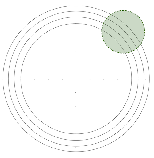
So with this base we now need to show that each of these elements (which are open sets) map to open sets when transformed via $f$ and conversely via $f^{-1}$.
For the open balls at the origin with radius $r$, we claim that they’ll continue to be open balls. To see why, consider the subset of points on an open ball at a fixed radius $r’ \lt r$. Since all these points have the same norm $r’$, the functions are just going to be a multiplication by a scalar $\alpha$, and we can use much the same ideas from Example 2 to see it gets transformed into an open ball with radius $r \alpha$.
For the open arcs of circumferences, we note that since all the points are at distance $r$ from the origin, they have the same norm and thus end up being transformed into a circumference of a different radius like above, and each open arc is still an open arc in this new circumference. QED.
We can show that the unit open ball is homemorphic to open balls of any size using a similar idea. At first glance it seems like using this idea we can prove any $n$-d “shape” is homeomorphic to $\mathbb{R}^n$ but we run into some trouble.
Consider an example in 2 dimensions. Suppose that instead of a circle we had a square centered at the origin. When mapping open balls from $\mathbb{R}^2$ into the square, to make sure they are inside, we have to choose a radius $r$ such that the corresponding open circle is inscribed in the square. But then there are parts of the square that would be unreacheable via this mapping, meaning that such mapping would not be bijective.
We’ll see next that the open square is also homeomorphic to $\mathbb{R}^2$ or more generally a bounded polytope is homeomorphic to $\mathbb{R}^n$.
Example 4: The $n$-dimensional bounded open convex polytope and open balls
A $n$-dimensional polytope is a general version of a polygon. A convex polytope is one that can be formed by the intersection of semi-planes, which can be succintly represented as:
\[Ax \le b\]This looks like the constraints of a linear programming model (LP). In fact a convex polytope is the feasible region of a LP. If we restrict the constraints to strict inequality:
\[Ax \lt b\]We get an open convex polytope. Note that the feasible region of a LP can be unbounded, for example one composed of a single constraint. If we restrict the cases where the area (or the corresponding measure for $n$ dimensions) to be finite, we have a bounded open convex polytope. As an example, a square without its borders is a bounded open convex polytope in 2D.
We shall now prove that a bounded open convex polytope $P$ that contains the origin is homeomorphic to an open ball centered at the origin.
Let’s consider the set of rays emanating from the origin. More formally, consider the set corresponding to the circumference of radius 1, $C = \curly{x \in \mathbb{R}^n$ \mid \norm{x} = 1}$. A ray of $c \in C$, denoted by $R_c$, is the set of points in the line that starts at the origin and passes by $c$, that is, the set $\curly{c\lambda, \lambda \gt 0}$ (note the rays don’t include the origin).
Let $P_B$ be the border (see precise definition in Closed Set, Limit Points, Closure, Border) of $P$. Because $P$ is convex, bounded and contains the origin, every ray $R_c$ is incident to exactly one point $v \in P_B$. For each $x \in R_c$, let $d(x) = \norm{v}$.
Let $B$ be the unit open ball at the origin. We can now define our homeomorphism. Let $f: B \rightarrow P$ be defined as:
\[f(x) = x d(x)\]If $x = 0$, define $f(0) = 0$. Conversely, the inverse function $f^{-1}: P \rightarrow B$ is:
\[f^{-1}(v) = \frac{v}{d(v)}\]To show open sets correspond to open sets when transformed by either function, we’ll define a new base as we did in Example 3. We’ll divide our base into two sets.
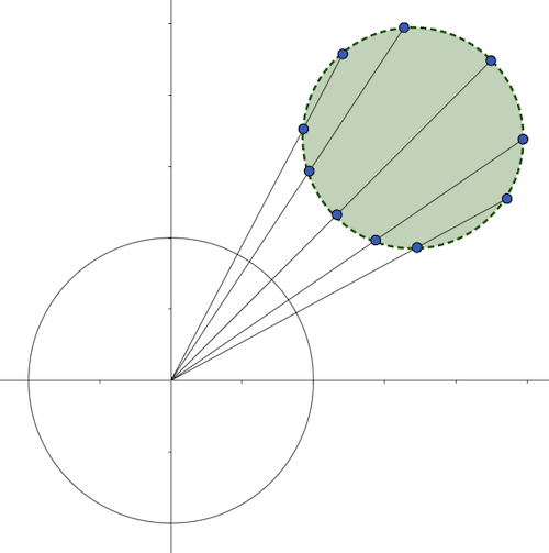
For an open ball that does not contain the origin, it’s the union of the open segments of $R_c$ for all $c \in C$, corresponding to the intersection of the ray and the open ball, which is an open segment, as depicted in Figure 3 for 2 dimensions. As in Example 3, a single segment is one dimensional and not an open set. We can add some width to them by bundling adjacent segments together and add them to our base.
For an open ball that contains the origin, we cannot cover with it only with rays because rays do not contain the origin. However, we if can include open balls centered at the origin it can be unioned with the thick rays to “plug” the hole at the origin.
For a given ray $R_c$, applying it over $f$ or $f^{-1}$ corresponds to scaling it by a fixed constant $d(c)$, so the result is an open segment, reasoning much like we did for open intervals in Example 1.
For a ball at the origin with radius $r$, when we apply $f$ to it, we’ll obtain the open convex polytope $P$ scaled by $r$. If we apply $f^{-1}$ to it, we’ll have an open bounded polytope that is however not convex, but is nevertheless open. QED.
In [7] Stefan Geschke proves the more general case where the open convex polytope need not be bounded.
It should be easy to find a homeomorphism between a polytope and its translatation by a fixed amount, so the restriction we started with of a polytope having to contain the origin is not a problem.
We can conclude that all open convex bounded polytopes are homeomorphic to the unit open ball and from Example 3, to $\mathbb{R}^n$.
Patterns in proving homeomorphisms
To prove the homeomorphism between 2 topological spaces $(X, \tau)$ and $(Y, \tau’)$, first we need to find a bijective function between $X$ and $Y$.
Then we try to find a suitable base whose elements can be transformed more conveniently. For Example3, since the function is based on the norm $\norm{x}$, it’s convenient to have in the base elements that have constant $\norm{x}$, for example arcs in a circumference at the origin.
Similarly in Example 4, the function depends on the function $d$ which is constant for points on the same ray $R_c$, so using elements along rays is convenient.
Conclusion
In this post we attempted to provide some formalism around the concept of topological equivalence. Trying to understand the homeomorphism between specific surfaces in 1D and 2D was rewarding and am very glad to sites like Mathematics Stack Exchange [3, 4, 5, 7] since these are not covered in the book I used as reference [1].
After studying the proofs I have a much better grasp on what it means when we say that topology is preserved under not only under rotation, translation but also stretching.
I still don’t know how to prove that a mug and a doughnut are topologically equivalent but I’ll leave it for another time.
Since topology has a lot of concepts and formal definitions, I also wrote a cheat sheet for reference.
Related Posts
- An Introduction to Matroids - There seems to be an apparent parallel between topological spaces $(X, \tau)$ and matroids $(E, \cal I)$. Both $X$ and $E$ are sets and both $\tau$ and $\cal I$ are collections of subsets satisfying some property. I wonder if there’s any more to them.
References
- [1] Introduction to Topology, Bert Mendelson
- [2] NP-Incompleteness: Hilbert Spaces
- [3] Mathematics Stack Exchange: Prove that some topology is not metrizable, Tomasz Kania.
- [4] Mathematics Stack Exchange: Prove that $(a, b)$ is homeomorphic to $(0,1)$, KonKan
- [5] Mathematics Stack Exchange: Is an open $n$-ball homeomorphic to $\mathbb{R}^n$? user149792
- [6] Wikipedia: Base (Topology)
- [7] Mathematics Stack Exchange: Proof that convex open sets in $\mathbb{R}^n$ are homeomorphic? Stefan Geschke
