kuniga.me > NP-Incompleteness > Hilbert Spaces
Hilbert Spaces
26 Jun 2021
In this post we’ll study the Hilbert space, a special type of vector space that is often used as a tool in the study of partial differential equations, quantum mechanics, Fourier analysis [1].
We’ll first define a Hilbert Space from the ground up from basic linear algebra parts, then study some examples.
The Hilbert Vector Space
Closedness
When we say a set $S$ is closed under some operation, it means that the result of that operation also belongs to $S$.
For example, the set of natural numbers $\mathbb{N}$ is closed under addition since the sum of two natural numbers is also natural. On the other hand, it’s not closed under subtraction, since the result might be a negative number.
Vector Space
Let $V$ be a set of vectors and $F$ a set of scalars. They define a vector space if $V$ is closed under addition and scalar multiplication from elements in $F$, which is known as a scalar field or simply field and usually is $\mathbb{R}$ or $\mathbb{C}$.
By this we mean that if $\vec{x}, \vec{y} \in V$, then $\vec{x} + \vec{y} \in V$, and that if $\vec{x} \in V, \alpha \in F$, then $\alpha \vec{x} \in F$.
One example of vector space is $V = \mathbb{R}^3$ and $F = \mathbb{R}$.
Inner Product Space
The inner product is a function from two vectors to a scalar and is denoted by $\langle \vec{x}, \vec{y} \rangle$, which must satisfy the following properties:
Let $\vec{x}, \vec{y}, \vec{z} \in V$ be vectors and $\alpha \in F$.
Linearity of the first argument:
- $\langle \alpha \vec{x}, \vec{y} \rangle = \alpha \langle \vec{x}, \vec{y} \rangle$
- $\langle \vec{x} + \vec{y}, \vec{z} \rangle = \langle \vec{x}, \vec{z} \rangle + \langle \vec{y}, \vec{z} \rangle$
Conjugate symmetry:
- $\langle \vec{x}, \vec{y} \rangle = \overline{\langle \vec{x}, \vec{y} \rangle}$
Positive definiteness:
- $\langle \vec{x}, \vec{x} \rangle > 0 \mbox{ if } \vec{x} \neq 0$
If our vector space is also closed under the inner product, it’s called a inner product space.
One example of inner product space is the Euclidean vector space, where $V = \mathbb{R}^n$, $F = \mathbb{R}$ and the inner product is the dot product,
\[\langle \vec{x}, \vec{y} \rangle = \vec{x} \cdot \vec{y} = \sum_{i=1}^n x_i y_i\]We can also define it for complex vector spaces, $V = \mathbb{C}^n$, $F = \mathbb{C}$ with inner product defined as
\[\langle \vec{x}, \vec{y} \rangle = \sum_{i=1}^n \bar{x_i} y_i\]where $\bar{x_i}$ is the complex conjugate of $x_i$.
Normed Space
A normed space is defined over a set of vectors $V$ and a norm operator denoted by $ \norm{\vec{x}}$, which can be interpreted as the length of a vector. The norm must satisfy:
Positive definiteness:
- $\norm{\vec{x}} \ge 0$ and $0 \mbox{ iff } \vec{x} = 0$
Positive homogeneity:
- $\norm{ \alpha \vec{x}} = \alpha \norm{\vec{x}}$
Subadditivity (Triangle inequality):
- $\norm{\vec{x} + \vec{y}} \le \norm{\vec{x}} + \norm{\vec{y}}$
We can show that every inner product space is a normed space. The inner product can be used to define a norm for a vector:
\[(1) \qquad \norm{\vec{x}} = \sqrt{\langle \vec{x}, \vec{x} \rangle}\]Metric Space
A metric space is defined over a set of vectors $V$ and a metric, a function that can be interpreted as the distance between two vectors and denoted by $d(\vec{x}, \vec{y})$, satisfying:
Positive definiteness:
- $d(\vec{x}, \vec{y}) \iff x = y$
Symmetry:
- $d(\vec{x}, \vec{y}) = d(\vec{y}, \vec{x})$
Subadditivity (Triangle inequality):
- $d(\vec{x}, \vec{z}) \le d(\vec{x}, \vec{y}) + d(\vec{y}, \vec{z})$
We can show that every normed space is a metric space, since we can define the metric from the norm as:
\[d(\vec{x}, \vec{y}) = \norm{\vec{x} - \vec{y}}\]Let’s now take a quick detour from vector spaces to cover Cauchy sequences and convergence. They’re an important concept used to define completeness, which we’ll see later.
Convergent Sequences
A sequence $x_1, x_2, x_3 \cdots \cdots$ converges to a limit $L$ if for any value $\varepsilon$, there exists $N$ such that for every $n \ge N$ such that
\[|x_n - L| < \varepsilon\]A sequence is convergent if it has a finite limit $L$.
Cauchy Sequences
A sequence $x_1, x_2, x_3 \cdots \cdots$ is a Cauchy sequence if for any value $\varepsilon$, there exists $N$ such that for every $n, m \ge N$,
\[\abs{x_n - x_m} < \varepsilon\]Let’s consider the sequence $\sqrt{n}$ for $n = 1, 2, \cdots$. Since consecutive values of $\sqrt{n}$ get closer and closer to each other as $n$ grows, for any $\varepsilon$ we can find $n$ such that $\abs{\sqrt{n + 1} - \sqrt{n}} < \varepsilon$. However, this has to hold for all indices above some $N$, and since $\sqrt{n}$ is unbounded, the difference between $\abs{\sqrt{n} - \sqrt{m}}$ for $n, m \ge N$ can be arbitrarily large, so this is not a Cauchy sequence.
One example of a Cauchy sequence is the sequence defined by $\frac{1}{n}$ for $n = 1, 2, \cdots$. Given some $\varepsilon$, we can find $N$ such that $\frac{1}{N} < \varepsilon$. This means that for $n, m \ge N$, $\frac{1}{n} < \varepsilon$ and $\frac{1}{m} < \varepsilon$, so their absolute difference also has to be bounded by $\varepsilon$.
Limit of a Cauchy sequence. Since we can choose an arbitrarily small value for $\varepsilon$, we can consider it tending to 0. Then
\[\lim_{\varepsilon \rightarrow 0} x_n = x_m = L \qquad \forall n, m \ge N\]Which means all Cauchy sequences are convergent.
Complete Metric Space
We can adapt the definition of Cauchy sequences for a metric space $(V, d)$. A sequence is formed by elements from $V$, that is $x_1, x_2, \cdots$ for $n = 1, 2, \cdots$ and $x_n \in V$. Such a sequence is Cauchy if there is $N$ such that for any $\varepsilon$, $d(x_n, x_m) < \varepsilon$ for $n, m \ge N$.
Let $M$ be the limit of a given Cauchy sequence $S$ in $(V, d)$. If for any $S$ the limit $M \in V$, then we say this metric space is complete. It’s worth noting that even though the result of $d$ is in $\mathbb{R}$, the limit of a sequence has a similar “shape” as elements in $S$.
One example of complete metric space is $V = \mathbb{R}$ with metric as the modulus operation and so is $V = \mathbb{R}^n$ with $d$ as the Euclidean distance.
One example that is not a complete metric space is $V = \mathbb{Q}$, the set of rationals, with metric as the modulus operation. To show that, we just need to find one Cauchy sequence that provides a counter-example. One such sequence is $x_1 = 1$ and $x_{n+1} = \frac{x_n}{2} + \frac{1}{x_n}$. We can show this is a Cauchy sequence and then find the limit by setting $x_{n+1} = x_n$, which yields $\sqrt{2}$, which is a irrational number and hence not in $V$.
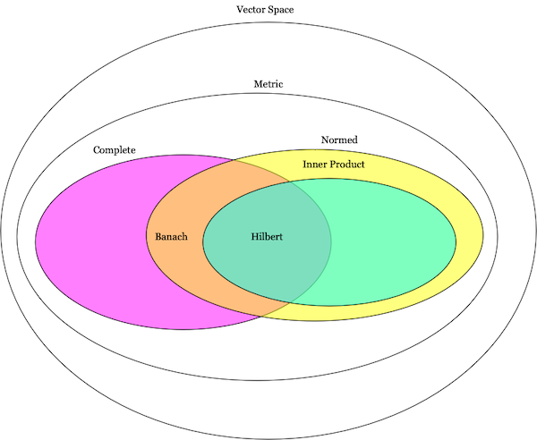
Hilbert space
Having gone through a bunch of different vector spaces, we are ready to define the Hilbert space, which is essentially a inner product space and a complete metric space.
A very similar space is the Banach space which is a normed space and a complete metric space. Note that since an inner product can be used to define a norm (as we saw in Metric Space), a Hilbert space is also a Banach space, but the opposite is not necessarily true.
Bases of Hilbert Spaces
We’ll now define the concept of bases for Hilbert spaces. Henceforth we’ll denote a Hilbert space by $H$.
But before we start, let’s take a quick detour into topology.
Dense Sets
A set $S$ is considered closed if it contains all its limit points. One convenient way to characterize this in our case is that all convergent sequences have their limit in $S$ [3].
For example, the set of real numbers in the closed interval $[0, 1]$ is closed, whereas those from the open interval $]0, 1[$ is not, because the sequence $\frac{1}{n}$ has a limit 0, and 0 does not belong to it.
The closure of a set $S$, which we’ll denote by $\bar S$ is $S$ plus the set of all its limit points. Another way to define closure is that it’s the smallest closed set that contains $S$ [4].
A subset $A$ of $S$ is called dense in $S$ if every point in $x \in S$ is either in $A$ or it’s one of its limit points [5]. In other words $S$ is the closure of $A$. For example, the set of rationals $\mathbb{Q}$ is dense in $\mathbb{R}$, because every real number can be approximated to be arbitrarily close to a rational.
Complete vs. Closed Metric Spaces
It’s worth clarifying the difference between closedness and completeness in the context of metric spaces. As we saw, a complete metric space $M$ is “closed” under the Cauchy sequences, meaning that the limit of Cauchy sequences belongs to $M$.
We can say a closed metric space $M$ is one “closed” under convergent sequences, meaning that the limit of convergent sequences belongs to $M$.
All Cauchy sequences are convergent, so a complete metric space is also a closed metric space.
Orthonormal Sets
Two vectors are orthogonal if their inner product equal to 0. More precisely, if $\vec{u}, \vec{v} \in H$ and $\langle \vec{f}, \vec{g} \rangle = 0$ then $\vec{u}$ and $\vec{v}$ are orthogonal, also denoted by $\vec{u} \perp \vec{v}$.
A subset $B \in H$ is orthonormal if all its elements are orthogonal and have unitary norm, that is $\forall \vec{u}, \vec{v} \in H$, $\vec{u} \perp \vec{v}$ and $\norm{\vec{u}} = 1$.
Orthonormal Bases
A set $B \in H$ is an orthonormal basis if it’s an orthonormal set and it’s complete. The latter means that the linear span $Sp$ of $B$ is dense in $H$.
To unpack that a bit, the linear span of $B$ is defined as:
\[Sp(B) = \bigg \{ \sum_{i=1}^{k} \lambda_i v_i | k \in \mathbb{N}, v_i \in B, \lambda_i \in F \bigg \}\]Where $F$ is a scalar field. A set $B$ is said complete if $\overline{Sp(B)} = H$.
Dimension
The dimension of a space is the size of any of its bases. Because Hilbert spaces admit infinite dimensional vectors, it’s possible that the dimension is infinite!
We’ll restrict ourselves to cases where the dimensions are countable, which is more general than the finite case [2].
It’s possible to show that $H$ having a countable orthonormal base is equivalent to it being separable, that is, there is countable subset $S$ dense in $H$.
Vector from Base
Like in linear algebra, we can write any vector in $H$ as a linear combination of the vectors in the base $B$, $\vec{v_1}, \vec{v_2}, \cdots$:
\[(2) \quad \vec{x} = \sum_{i=1}^{\infty} \lambda_i \vec{v_i}\]Conversely the coefficients correspond to:
\[(3) \quad \lambda_i = \langle \vec{v_i}, \vec{x} \rangle\]Parseval’s identity
The coefficients from the base above can be used to compute the norm of $\vec{x}$, like in linear algebra:
\[(4) \quad \norm{\vec{x}}^2 = \sum_{i=1}^{\infty} \abs{\lambda_i}^2\]This is known as the Parseval’s identity. We can arrive at this identity by recallling that the norm can be obtained from the inner product as (1):
\[\norm{\vec{x}} = \sqrt{\langle \vec{x}, \vec{x} \rangle}\]or
\[\norm{\vec{x}}^2 = \langle \vec{x}, \vec{x} \rangle\]if we replace the first $\vec{x}$ by (2),
\[\norm{\vec{x}}^2 = \langle \sum_{i=1}^{\infty} \lambda_i \vec{v_i}, \vec{x} \rangle\]since inner product is linear on the first argument, we can move the sum and the scalar factor out:
\[\norm{\vec{x}}^2 = \sum_{i=1}^{\infty} \lambda_i \langle \vec{v_i}, \vec{x} \rangle\]we can then use the conjugate symmetry property to get:
\[\norm{\vec{x}}^2 = \sum_{i=1}^{\infty} \lambda_i \overline{\langle \vec{v_i}, \vec{x} \rangle}\]and then replace it by (3):
\[\norm{\vec{x}}^2 = \sum_{i=1}^{\infty} \lambda_i \overline{\lambda_i}\]which then leads to (4). Another way to state Parseval’s identity is to replace $\lambda_i$ with $\langle \vec{v_i}, \vec{x} \rangle$ instead of the opposite, which leads to:
\[\norm{\vec{x}}^2 = \sum_{i=1}^{\infty} \abs{\langle \vec{v_i}, \vec{x} \rangle}^2\]Bessel’s inequality
Bessel’s inequality is a generalization of Parseval’s:
\[\norm{\vec{x}}^2 \ge \sum_{i=1}^{N} \abs{\lambda_i}^2\]It follows naturaly from the fact that the interval $[1, N]$ is a subset of $[1, \infty]$.
Orthogonal Complement
Let $S$ be a closed subspace of $H$. Its orthogonal complement is defined as
\[S^{\perp} = \{\vec{y} \in H | \langle \vec{y}, \vec{x} \rangle = 0, \, \forall \vec{x} \in S \}\]An example for some geometric intuition could be for the $\mathbb{R}^3$, with $S$ being the vectors in the xy plane, that is, those with $z = 0$. Then $S^{\perp}$ would be those perpendicular to the xy plane ($x = y = 0$).
Orthogonal Projection
Let $S$ be a closed subspace of $H$. The orthogonal projection of $\vec{x}$ onto $S$ is a vector $\vec{x_S}$ that minimizes the distance from $\vec{x}$ to $S$. Note that $\vec{x}$ does not need to be in $S$.
More formally, it’s
\[(5) \quad \vec{x_S} = \mbox{argmin}_{\vec{y} \in S} \norm{\vec{x} - \vec{y}}\]It’s possible to prove $x_S$ exists and is unique.
Going back to our geometry example, the orthogonal projection of a vector $(x, y, z)$ onto $z = 0$ is the vector $(x, y, 0)$.
The Projection Theorem
Let $S$ be a closed subspace of $H$. The theorem states that every $\vec{x} \in H$ can be written as $\vec{x} = \vec{x_S} + \vec{x}^{\perp}$, where $\vec{x_S}$ is the orthogonal projection of $\vec{x}$ onto $S$ and $\vec{x}^{\perp} \in S^{\perp}$.
Going back to our geometry example, we can say that every vector in $\mathbb{R}^3$ can be expressed as the sum of a vector in the xy-plane and a vector perpendicular to it, or more specifically, $\vec{x} = (x, y, z)$, $\vec{x_S} = (x, y, 0)$ and $(0, 0, z) \in S^{\perp}$.
Least Square Approximation via Subspaces
The idea is to approximate a vector with infinite dimension by one with finite one. Recall from (2) that for any $\vec{x} \in H$ and base $\vec{v_1}, \vec{v_2}, \cdots$:
\[\quad \vec{x} = \sum_{i=1}^{\infty} \lambda_i \vec{v_i}\]We can approximate $\vec{x}$ by taking the first $N$ terms, which we’ll denote by $\vec{x}^{[N]}$:
\[\quad \vec{x}^{[N]} = \sum_{i=1}^{N} \lambda_i \vec{v_i}\]It’s possible to show that $\vec{x}^{[N]}$ is a orthogonal projection of $\vec{x}$ onto $V_N = Sp(\vec{v_1}, \vec{v_2}, \cdots, \vec{v_N})$. Thus, by (5):
\[\norm{\vec{x} - \vec{x}^{[N]}} = \min \{\norm{\vec{x} - \vec{y}} \mid \vec{y} \in V_N \}\]since $y \in V_N$, $y = \sum_{i=1}^{N} \alpha_i \vec{v_i}$. We can define an error function taking $\alpha_i$ as parameter:
\[E_N(\alpha_1, \cdots, \alpha_N) = \norm{\vec{x} - \sum_{i=1}^{N} \alpha_i \vec{v_i}}\]The idea is then to find the value of $\alpha$’s that minimize ${E_N}^2$ (least squares).
Examples
Finite Euclidean Spaces
We’ve seen that the Euclidean vector space is a inner product space (see Inner Product Space) and a complete metric space (see Complete metric space), so it’s a Hilbert space by definition.
Polynomial Functions
Most of the times when we talk about vector spaces we use scalars or vectors of scalars as examples, but nothing stops us from using other types of objects like functions. We can have a vector space of polynomial functions for example.
A polynomial function of degree $N$ takes a variable $x$ and returns a polynomial $\sum_{i = 0}^{N} \alpha_i x^i$ where $\alpha_i$ is a scalar from an interval $[a, b]$. The set of polynomial functions of degree $N$ over a field $F$ can be denoted as $\mathbb{P}_N(F)$.
The inner product of two polynomial functions $\vec{f}$ and $\vec{g}$ can be defined as:
\[\langle \vec{f}, \vec{g} \rangle = \int_a^b \overline{f(x)} g(x) dx\]This function is also known as $L^2[a, b]$. It’s possible to show that the vector space $(\mathbb{P}_N(F), L^2[a, b])$ is a Hilbert one.
Square Summable Sequences
One interesting advantage of building vector spaces based on properties like inner product instead of working directly with the actual vectors is that we can have vector spaces with infinte dimensions!
Let $\mathbb{C}^{\infty}$ be the set of complex vectors with infinite dimensions and inner product:
\[\langle \vec{x}, \vec{y} \rangle = \sum_{i=1}^{\infty} \bar{x_i} y_i\]From that we can define the norm as:
\[\norm{\vec{x}} = \sum_{i=1}^{\infty} \abs{x_i}^2\]Let $\ell^2$ be the subset of $\mathbb{C}^{\infty}$ for those that have finite norm, that is:
\[\ell^2 = \{ \vec{x} \in \mathbb{C}^\infty \mid \sum_{i=1}^{\infty} \abs{x_i}^2 < \infty \}\]$\ell^2$ is also known as square summable sequences, since the elements of \(\vec{x} \in \ell^2\) form a sequence that has a finite square sum.
It’s possible to show \(\ell^2\) is a Hilbert space.
Conclusion
In this post we covered some topics around Hilbert spaces. I’m mostly interested in definitions and theorems, so I ended up skipping their proofs. Although there’s some geometric intuition to it, a lot of the content is still a bit over my head, and I’m hoping studying some of the applications in the future will help clarify things.
My main motiviation in studying these topics is to better understand the mathematics of signal processing. I’ve started reading Prandoni and Vetterli’s Signal Processing for Communications [6] where they first discuss Hilbert spaces.
This is my first foray into functional analysis and topology and it felt very hard to understand, but I love how much available material there is about this subject freely available on the internet [2]!
