kuniga.me > NP-Incompleteness > Discrete Time Filters
Discrete Time Filters
31 Aug 2021
In this post we’ll learn about discrete filters, including definitions, some properties and examples.
Discrete Filter
A discrete-time system is a transform that takes in discrete-time sequences as inputs and produces another discrete-time sequence at its output. In the general case we can think of it as a function $\mathscr{H}$ from a vector $\vec{x}$ to another vector $\vec{y}$ that is also dependent on the time parameter $t$:
\[y_t = \mathscr{H}(\vec{x}, t)\]Note: the input of the function is $\vec{x}$, not $x_t$ because $y_t$ could depend on more than just $x_t$, for example a window function where $y_t = x_{t-1} + x_{t} + x_{t+1}$.
A discrete-time system is said linear if it satisfies:
\[\mathscr{H}(\alpha \vec{x} + \beta \vec{y}, t) = \alpha \mathscr{H}(\vec{x}, t) + \beta \mathscr{H}(\vec{y}, t)\]A discrete-time system is said time-invariant if it doesn’t actually depend on $t$. That is, if we shift the signal $x$ (by adding a delay $\Delta$), the output is also shift but doesn’t change.
In [2] the authors provide a good example to make this distinction clear. A transform $\mathscr{H}(x_t, t) = t x_t$ is time-variant, because if we shift $\vec{x}$ by $1/2$ the output doesn’t simply shift, it changes “shape”.
On the other hand $\mathscr{H}(x_t, t) = x^2_t$ is time-invariant, since the output for the shifted $\vec{x}$ is basically $\vec{y}$ shifted by the same amount.
A discrete-time system that is both linear and time-invariant (also known as LTI) is what we call a discrete filter. We’ll focus on discrete filter in this post, so henceforth we’ll assume $\mathscr{H}$ is an LTI function.
Convolution
The impulse response
An impulse signal $\delta$ is a vector filled with all zeros except the entry $t = 0$ which is 1.
The result of applying a discrete filter $\mathscr{H}$ over $\delta$ is called an impulse response, often denoted as $h$:
\[h_t = \mathscr{H}(\delta, t)\]The Reproducing Formula
We can obtain an entry for vector $\vec{x}$ at $t$ by multiplying itself with $\delta$:
\[(1) \quad x_t = \sum_{k = -\infty}^{\infty} x_k \delta_{t - k}\]which is known as the reproducing formula. To see why this identity is true, we observe that the only case in which $\delta_{t - k}$ is non-zero is when $k = t$.
Convolution Operator
We can apply $\mathscr{H}$ over (1) to get $y_t$:
\[y_t = \mathscr{H}(\vec{x}, t) = \mathscr{H}(\sum_{k = -\infty}^{\infty} x_k \delta_{t - k}, t)\]One key observation is that in (1), $x_k$ can be seen as the scalar multiplying the variable $\delta_{t - k}$ (though I’m not super sure on the rationale). Thus we can apply the linearity principle to obtain:
\[y_t = \sum_{k = -\infty}^{\infty} x_k \mathscr{H}(\delta_{t - k}, t) = \sum_{k = -\infty}^{\infty} x_k h_{t - k}\]This last sum is the definition of the convolution operator for a given index $t$, which is basically a inner product of infinite length vectors where one of the vectors have its index $k$ reversed ($-k$) and then shifted ($-k + t$).
We can define the convolution at the vector level, in which case it can be more simply stated using a the $*$ symbol:
\[\vec{y} = \vec{x} * \vec{h}\]We can now observe that a filter $\mathscr{H}$ can be fully described by the vector $h$.
Properties
If the input is a square summable sequence, it’s possible to show the convolution operator is associative:
\[(\vec{x} * \vec{h}) * \vec{w} = \vec{x} * (\vec{h} * \vec{w})\]If $\vec{h}$ and $\vec{w}$ are the impulse responses of filters $\mathscr{H}$ and $\mathscr{W}$, this implies there exists a filter whose impulse response is $(\vec{h} * \vec{w})$ which is equivalent to passing $\vec{x}$ through filters $\mathscr{H}$ and then $\mathscr{W}$.
The convolution operator is commutative, so the order in which we apply filters is irrelevant.
Frequency Domain
Suppose we feed a filter an complex exponential signal, as defined in out previous post [3]:
\[x_t = A e^{i (\omega t + \phi)}\]We can obtain the output via a convolution:
\[\mathscr{H}(\vec{x}, t) = \vec{x} * \vec{h} = \sum_{k = -\infty}^{\infty} x_k h_{t - k}\]Since convolution is associative,
\[= \sum_{k = -\infty}^{\infty} h_{k} x_{t - k} = \sum_{k = -\infty}^{\infty} h_{k} A e^{i (\omega (t - k) + \phi)}\]Moving the factors that do not depend on $k$ out of the sum,
\[= A e^{i (\omega t + \phi)} \sum_{k = -\infty}^{\infty} h_k e^{- i \omega k}\]Now we recall the definition of DTFT as equation (6) from [3]:
\[\lambda(\omega) = \sum_{t = 0}^{N-1} x_t e^{-i \omega t} \quad 0 \le \omega \le 2 \pi\]With $N \rightarrow \infty$ and given it’s possible to show in this case that the sum over $[0, \infty]$ results in the same as $[-\infty, \infty]$, we can define $H(\omega)$ as the DTFT of the vector $\vec{h}$ and obtain:
\[(2) \qquad \mathscr{H}(\vec{x}, t) = A e^{i (\omega t + \phi)} H(\omega)\]$H(\omega)$ is also called the frequency response of the filter at frequency $\omega$.
Consider the polar form of $H(\omega)$ as:
\[H(\omega) = A_0 e^{i \theta_0}\]And we define amplitude as $\abs{H(\omega)} = \abs{A_0}$ and the phase is $\angle H(\omega) = \theta_0$. When we use this canonical form in (2) we get:
\[\mathscr{H}(\vec{x}, t) = A A_0 e^{i (\omega t + \phi + \theta_0)}\]Thus we can observe the filter scales the amplitude of the original signal by $A_0$ and shifts its phase by $\theta_0$.
Convolution and Modulation
Let $\vec{x}$ and $\vec{y}$ be two absolute summable vectors and $z = x * y$ their convolution. We show that the DFTF of $z$, $Z(\omega)$, is the product of the DFTF of $x$ and $y$, $Z(\omega) = X(\omega) Y(\omega)$, which is known as the convolution theorem.
Proof.
Let’s apply the DTFT over the expanded sum of the convolution:
\[Z(\omega) = \sum_{t = -\infty}^{\infty} \sum_{k = -\infty}^{\infty} x_k y_{t - k} e^{i \omega t}\]Since $\vec{x}$ and $\vec{y}$ are absolute summable, these sums are finite and can be swapped and their terms re-arranged:
\[= \sum_{k = -\infty}^{\infty} (x_k \sum_{t = -\infty}^{\infty} y_{t - k} e^{i \omega t})\]We can “borrow” a factor of $e^{i \omega k}$ from $e^{i \omega t}$ just to obtain the form we want:
\[Z(\omega) = \sum_{k = -\infty}^{\infty} (x_k e^{i \omega k} \sum_{t = -\infty}^{\infty} y_{t - k} e^{i \omega (t - k)})\]We can re-index $t$ as, say $t’ = t - k$, for any $k$, so that the infinite sum is preserved (see Appendix for a more formal argument), i.e.
\[\sum_{t = -\infty}^{\infty} y_{t - k} e^{i \omega (t - k)} = \sum_{t' = -\infty}^{\infty} y_{t'} e^{i \omega (t')}, \qquad k \in \mathbb{Z}\]Then we can obtain two independent sums:
\[Z(\omega) = (\sum_{k = -\infty}^{\infty} x_k e^{i \omega k}) (\sum_{t' = -\infty}^{\infty} y_{t'} e^{i \omega t'}) = X(\omega) Y(\omega)\]QED.
We can also show that the convolution of the DTFTs of $\vec{x}$ and $\vec{y}$ correspond to the DTFT of their product. That is, if $Z(\omega) = X(\omega) * Y(\omega)$, then $z_t = x_t y_t$, where the definition of the convolution for continuous functions is:
\[(3) \quad X(\omega) * Y(\omega) = \int_{0}^{2 \pi} X(\sigma) Y(\omega - \sigma) d\sigma\]This is known as the modulation theorem.
Proof.
Let’s recall the definition of the inverse of the DTFT (equation (5) in [3]):
\[x_t = \frac{1}{2 \pi} \int_{0}^{2 \pi} X(\omega) e^{i \omega t} d\omega\]Applying it for $Z(\omega)$:
\[z_t = \frac{1}{2 \pi} \int_{0}^{2 \pi} X(\omega) * Y(\omega) e^{i \omega t} d\omega\]Replacing (3) (commutative form):
\[= \frac{1}{2 \pi} \int_{0}^{2 \pi} \frac{1}{2 \pi} \int_{0}^{2 \pi} X(\omega - \sigma) Y(\sigma) e^{i \omega t} d\sigma d\omega\]Splitting $\omega$ into $(\omega - \sigma) + \sigma$:
\[= \frac{1}{2 \pi} \int_{0}^{2 \pi} \frac{1}{2 \pi} \int_{0}^{2 \pi} (X(\omega - \sigma)e^{i (\omega - \sigma)}) (Y(\sigma)) e^{i \sigma t}) d\sigma d\omega\]Given the periodic nature of the DFTF, shifting the indices by a given amount $\omega$ doesn’t change the result, so:
\[\int_{0}^{2 \pi} X(\sigma) e^{i \sigma t} d\sigma = \int_{0}^{2 \pi} X(-\sigma) e^{i (-\sigma) t} d\sigma = \int_{0}^{2 \pi} X(\omega - \sigma) e^{i (\omega - \sigma) t} d\sigma\]We can use this to obtain two independent sums:
\[z_t = (\frac{1}{2 \pi} \int_{0}^{2 \pi} X(\omega - \sigma) e^{i (\omega - \sigma) t} d\sigma) (\frac{1}{2 \pi} \int_{0}^{2 \pi} Y(\omega) e^{i \sigma t}d\omega)\]which correspond to \(x_t y_t\).
Properties
IIR vs FIR
The impulse response of a filter is always an infinite vector since the impulse vector is also infinite. The non-zeros entries on the impulse response are called taps.
Infinite-impulse response (IIR) are filters whose impulse responses have an infinite amount of taps, as opposed to finite-impulse response (FIR). The latter is a finite-support signal (recall it’s an infinite signal created by padding a finite one with 0s).
Causality
A causal filter is one that does not depend on the future, which means in $y_t = \mathscr{H}(\vec{x}, t)$, $y_t$ will only be defined in terms of $x_k$ for $k \le t$. So in
\[y_t = \sum_{k = -\infty}^{\infty} x_k h_{t - k}\]we want $h_{t - k}$ to be 0 if $k > t$. If we call $z = t - k$, then $k > t$ implies $z < 0$ and thus $h_z = 0$ for $z < 0$. In other words, $\vec{h}$ must zeroes for negative indices.
Causality is important in real-time systems, where we only have the signal up to the current timestamp $t$.
Stability
A system is called bounded-input bounded-output (BIBO) if the output is bounded when the input is bounded. By bounded we mean that each entry in the vector is finite, or more formally, there exists $L \in \mathbb{R}^{+}$ such that $\abs{x_n} < L$ for all $n$.
A necessary and sufficient condition for a filter to be BIBO is for its impulse response $\vec{h}$ to be absolutely summable.
Proof. For the sufficiency, suppose $\vec{h}$ is absolutely summable, that is,
\[\sum_{k = -\infty}^{\infty} \abs{h_k} < \infty\]We want to show $\abs{y_n}$ is bounded when $\abs{x_n}$ is bounded. We have
\[\abs{y_n} = \abs{\sum_{k = -\infty}^{\infty} x_k h_{t - k}} \le \sum_{k = -\infty}^{\infty} \abs{x_k h_{t - k}} = \sum_{k = -\infty}^{\infty} \abs{x_k} \abs{h_{t - k}}\]There exists some $L$ such that $\abs{x_n} < L$, so
\[\abs{y_n} < L \sum_{k = -\infty}^{\infty} \abs{h_{t - k}}\]And we started from the hypothesis the last sum is finite, so $\abs{y_n}$ is also finite.
For the necessity, we just need to show an example where $\vec{h}$ is not absolutely summable, $\vec{x}$ is bounded and $\vec{y}$ is not. We define $x_n = \mbox{sign}(h_{-n})$, that is $x_n \in \curly{-1, 0, 1}$ and thus bounded.
If we consider $\abs{y_t}$ for $t = 0$:
\[\abs{y_0} = \abs{\sum_{k = -\infty}^{\infty} x_k h_{-k}}\]The term $x_k h_{-k}$ is equal to $\abs{h_{-k}}$ (from our choice of $x_k$), so
\[\abs{y_0} = \sum_{k = -\infty}^{\infty} h_{-k}\]which we assumed is infinite. QED
Because FIR filters’ impulse response have a finite number of non-zero terms, they’re absolute summable, hence FIR filters are BIBO.
Magnitude
As we discussed earlier, the amplitude of the frequency response $H(\omega)$ scales the amplitude of the original signal when a filter is applied. The frequency response is a function which can return different amplitudes for different frequencies $0 \le \omega \le 2 \pi$, and can be thus used to boost certain frequencies and attenuate others.
We can categorize filters based on what types of frequencies it boosts (if any).
- Lowpass filters. The amplification is concentrated at low frequencies $\omega = 0 = 2 \pi$.
- Highpass filters. The amplification is concentrated at high frequencies $\omega = \pi$.
- Bandpass filters. The amplification is concentrated at specific frequencies $\omega_p$.
- Allpass filters. The amplification is uniform across the spectrum.
The names are very intuitive, the “pass” means what types of frequencies the filter allows passing through.
Phase
As we discussed earlier, the phase of the frequency response $H(\omega)$ corresponds to a shift on the frequencies of the input signal. In time domain, this corresponds to a delay.
Consider a sinusoidal signal, $x_t = e^{i (\omega t)}$ and let’s assume $t$ is continuous. Suppose we apply a filter with amplitude $A_0 = 1$ and phase $\theta_0$. Once we apply the filter we get $y_t = e^{i (\omega t + \theta_0)}$.
Using Euler’s identity, the real part of $y_t$ is $\cos (\omega t + \theta_0)$. If we define $t_0 = - \frac{\theta_0}{\omega}$, known as phase delay, we have $\cos (\omega (t - t_0))$. If we’re to plot this (continuous) function, we’ll see each point $x_t$ got delayed by an amount $t_0$ in $y_t$.
For the discrete time case, because we’re sampling at regular intervals that might not align with the delay, there might not be a 1:1 mapping between $x_t$ and $y_t$.
The frequency response $H(\omega)$ might have different phases for different frequencies $\omega$, thus each frequency of the input signal might be shifted by different amounts, so even if the filter has amplitude $A_0 = 1$, the “shape” of the output signal might be different.
Linear Phase. A linear phase filter is when its phase function $\angle H(\omega)$ is linear on $\omega$, that is, $\angle H(\omega) = \omega d$, $d \in \mathbb{R}$.
Assuming $A_0 = 1$, now the output signal is $y_t = e^{i (\omega (t + d))}$, thus the signal gets shifted by the same amount on all its frequency and the “shape” of the output would be the same as the input.
Locally Linear Phase. Even for non-linear phase filters, it’s possible to have approximately linear behavior around specific frequencies.
Consider a specific frequency $\omega_0$ and any other frequency $\omega$ around it, and $\omega - \omega_0 = \tau$. We can approximate $\angle H(\omega)$ by a linear function around $\omega_0$ by using a first order Taylor approximation:
\[\angle H(\omega_0 + \tau) = \angle H(\omega_0) + \tau \angle H'(\omega_0)\]We then have
\[H(\omega_0 + \tau) = \abs{H(\omega_0 + \tau)} e^{i \angle H(\omega_0 + \tau)} = (\abs{H(\omega_0 + \tau)} e^{i \angle H(\omega_0)}) e^{i \angle H'(\omega_0) \tau}\]We can see this as an extra phase shift of $\angle H’(\omega_0) \tau$. The negative of $\angle H’(\omega_0)$ is defined as the group delay.
Examples
Let’s consider two basic filters and investigate some of their properties.
Moving Average
A classic example of filter is the moving average, which consists of taking the average of the previous $N$ samples:
\[y_t = \mathscr{H}(\vec{x}, t) = \frac{1}{N} \sum_{k = 0}^{N - 1} x_{t - k}\]We can apply $\mathscr{H}$ to $\delta$ to obtain the impulse response:
\[h_t = \frac{1}{N} \sum_{k = 0}^{N - 1} \delta_{t - k}\]Recall that the only non-zero entry in $\vec{\delta}$ is when $t = k$, so the sum is $\frac{1}{N}$, unless the range $[0, N - 1]$ doesn’t include $t$, that is, if $t < 0$ or $t \ge N$, summarizing:
\[\begin{equation} h_t =\left\{ \begin{array}{@{}ll@{}} \frac{1}{N}, & \text{if}\ 0 \le t < N \\ 0, & \text{otherwise} \end{array}\right. \end{equation}\]which means it has a finite number of non-zero entries and thus $\mathscr{H}$ is a FIR filter. This specific definition of moving average is also causal.
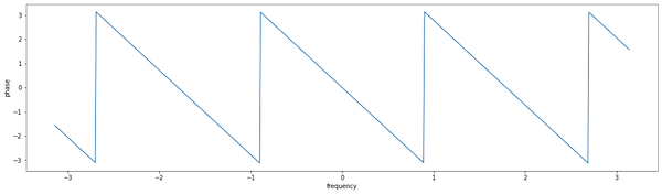
It’s possible to show that the frequency response of this filter is
\[H(\omega) = \frac{1}{N} \frac{\sin(\omega N/2)}{\sin(\omega / 2)} e^{-i \frac{N -1}{2} \omega}\]If we plot the amplitude (see Figure 3), we can see that it magnifies mostly low frequencies which matches that intuition that moving average smooths a signal, removing high-frequency noises.
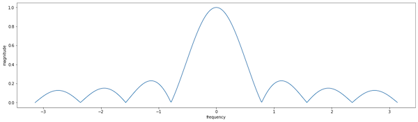
We can also plot the phase delay from above, which is $\frac{N-1}{2}$. It matches the intuition that when we average the last $N$ points the “center of gravity” is in the middle of this window.
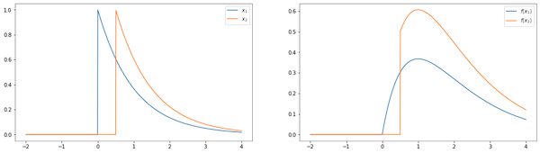
Leaky Integrator
Suppose we parametrize the moving average by the window size $N$:
\[\mathscr{H}_N(\vec{x}, t) = \frac{1}{N} \sum_{k = 0}^{N - 1} x_{t - k}\]We can then write $\mathscr{H}_{N}(\vec{x}, t)$ in terms of $\mathscr{H}_{N - 1}(\vec{x}, t - 1)$, noting that the latter is:
\[(4) \quad \mathscr{H}_{N -1 }(\vec{x}, t - 1) = \frac{1}{N - 1} \sum_{k = 0}^{N - 2} x_{t - 1 - k} = \frac{1}{N - 1} \sum_{k = 1}^{N - 1} x_{t - k}\]First we extract the first term out of the sum (i.e. the when $k = 0$):
\[= \frac{1}{N} (x_t + \sum_{k=1}^{N-1} x_{t - k})\]Normalizing the denominator of the second term to $N - 1$:
\[= \frac{1}{N} x_{t} + \frac{N - 1}{N} \frac{1}{N - 1} \sum_{k=1}^{N-1} x_{t - k}\]We can replace (4) here:
\[= \frac{1}{N} x_{t} + \frac{N - 1}{N} \mathscr{H}_{N - 1}(\vec{x}, t - 1)\]If we call $\lambda_N = \frac{N - 1}{N}$, then $\frac{1}{N} = 1 - \lambda_N$:
\[\mathscr{H}_{N}(\vec{x}, t) = \lambda_N \mathscr{H}_{N - 1}(\vec{x}, t - 1) + (1 - \lambda_N) x_{t}\]As $N$ becomes large, adding a term to the average changes little, so $\mathscr{H}_{N+1}$ and $\mathscr{H}_{N}$ become approximately the same. Thus, assuming a sufficiently large $N$ we can drop the $N$ parameter to get:
\[\mathscr{H}(\vec{x}, t) = \lambda \mathscr{H}(\vec{x}, t - 1) + (1 - \lambda) x_{t}\]or in terms of $\vec{y}$,
\[y_t = \lambda y_{t - 1} + (1 - \lambda) x_t\]This system is known as the leaky integrator. When $\lambda \rightarrow 1$, then $N \rightarrow \infty$, and this filter is simply the sum of the terms of $\vec{x}$, thus an integrator. Since in reality it is not exactly 1, it doesn’t account for all the terms, so it “leaks”.
It’s possible to show this is a LTI system (a filter), if we add a condition that $y_n$ “starts somewhere”, that is, before a instant $t_0$, all its entries are zero:
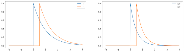
\[y_t = 0, \qquad t < t_0\]In particular, we’ll assume $t_0 = 0$, which simplifies calculations. We can apply this filter to $\vec{\delta}$ to get an impulse response. We have for $t = 0$:
\[h_0 = (1 - \lambda) \delta_0 = 1 - \lambda\]For $t > 0$, since $\delta_t = 0$, we have
\[h_t = \lambda h_{t-1}\]Which gives us a closed form:
\[h_t = (1 - \lambda) \lambda^t, \qquad t \ge 0\]This shows this impulse response is infinite, thus the leaky integrator is an IIR filter.
It’s possible to show that the frequency response of this filter is
\[H(\omega) = \frac{1 - \lambda}{1 - \lambda e^{-i \omega}}\]With magnitude:
\[\abs{H(\omega)} = \frac{(1 - \lambda)^2}{1 + \lambda^2 - 2\lambda \cos(\omega)}\]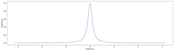
and phase:
\[\angle H(\omega) = \arctan \left(-\frac{\lambda \sin(\omega)}{1 - \cos(\omega)}\right)\]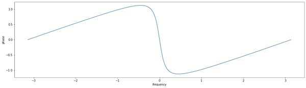
Appendix
In Convolution and Modulation we claimed that we can shift the index $t$ in an infinite sum by an arbitrary amount $k \in \mathbb{Z}$, that is, given $t’ = t - k$:
\[\sum_{t = -\infty}^{\infty} f(t) = \sum_{t' = -\infty}^{\infty} f(t')\]Let’s call $T$ the set of indices corresponding to $[-\infty, \infty]$, i.e. $T$ is the set of integers $\mathbb{Z}$.
In the second sum we have $t’ = t - k \in [-\infty, \infty]$ or $t \in ([-\infty, \infty]) + k$, which we’ll call $T’$. $T’$ is basically $T$ with all elements plus $k$, so for every $t \in T$, there’s exactly one $t + k \in T’$. Since $k \in \mathbb{Z}$ and $\mathbb{Z}$ is closed under addition, $t + k \in \mathbb{Z}$, so every element in $T’$ exists in $T$ as well, or that if $t \in T$ then $t \in T’$.
Conversely we can show that if $t’ \in T’$ then $t’ \in T$. For every $t’ \in T$ there’s exactly one $t’ - k \in T$ and $\mathbb{Z}$ is closed under subtraction, so $t’ \in T$ as well.
We conclude that there’s a one-to-one mapping between $T$ and $T’$ and thus the sums are over the same set of indices. QED.
Conclusion
As in Discrete Fourier Transforms we used a different notation than the usual in signal processing.
I learned a bunch of things from this post, including: convolution, the leaky integrator, the formalism behind the “delay” from moving average filters.
Related Posts
- Linear Predictive Coding in Python. We ran into convolution in The LPC Model section. Note that the filter is denoted by $h_t$ like we did here, which is not a coincidence. I also realize I’ve been studying things backwards :)
References
- [1] Signal Processing for Communications, Prandoni and Vetterli
- [2] Linearity, Causality and Time-Invariance of a System
- [3] Discrete Fourier Transforms
All the charts have been generated using Matplotlib, the source code available as a Jupyter notebook.
