kuniga.me > NP-Incompleteness > Viterbi Algorithm
Viterbi Algorithm
25 Jan 2021

Andrew Viterbi is an Italian-born American electrical engineer who co-founded Qualcomm and is also known for the Viterbi algorithm, although the method has been independently discovered by other people [1].
His family fled Italy due to Mussolini’s fascist policies which targeted Italy’s Jewish population [2]. He obtained his BS and MS from MIT and PhD from USC (University of Southern California), whose School of Engineering is named after Andrew and his late wife Erna.
In this post we’ll discuss the Viterbi algorithm in the context of Hidden Markov Models
Hidden Markov Model
We can think of a Hidden Markov Model as a probabilistic state machine. We are given a graph with nodes corresponding to hidden (or latent) states and edges corresponding to transitions between states, associated with a probability of going from one state to another.
Associated with each node is a set of possible visible states, or observations, which act as a proxy to the hidden state. There’s a probability of observing a visible state given a hidden state.
Let’s go into more details and introduce more formal notation.
States. There are $N$ (hidden) states in the model, $S = \curly{s_1, s_2, \cdots, s_N}$. Each node correspond to one of these states.
Time. As in a state machine, we have the concept of time. At any given instant $t$, we are in a state (or node) $q_t$. We start at $t = 0$ at any given state $q_0 = s_i$ with probability $\pi_i$ for $i \in \curly{1, 2, \cdots, N}$.
Transition. When going from instant $t$ to $t+1$, we make a state transition. The probability of going to state $s_j$ given we’re at a state $s_i$ is given by the variable $a_{ij}$, where
\[\sum_{j = 1}^{N} a_{ij} = 1 \qquad \forall i \in \curly{1, 2, \cdots, N}\]Note that we may end up staying on the same state if $a_{ii} > 0$.
The $N \times N$ matrix of $a_{ij}$ is denoted by $A$. The “Markov” in “Hidden Markov Model” stems from the fact that the probability of transition only depends on the current state, that is, independent from the past like in a Markov chain.
Observation. The “Hidden” in “Hidden Markov Model” models the fact that it might be hard or impossible to directly measure or observe a state $s_i$, and instead we use a proxy metric or observation that is ideally highly correlated with $s_i$.
There are $M$ observable states in the model, $V = \curly{v_1, v_2, \cdots, v_M}$. The probability of observing $v_k$ given we’re in state $s_i$, $p(v_k \mid s_i)$, is encoded in the variable $b_{ik}$. The $N \times M$ matrix of $b_{ik}$ is denoted by $B$.
Estimating the Hidden States Sequence
Suppose we have a sequence of observations $O = o_1, o_2, \cdots, o_T$, where $o_i \in \curly{v_1, \cdots v_M}$ and a model with all the variables $(S, V, A, B, \pi)$ defined. We want to estimate the sequence of hidden states most likely to have yielded such observations.
More formally, let $Q = q_1, q_2, \cdots, q_T$ be a sequence of states where $q_i \in \curly{s_1, \cdots s_N}$. The probability of observing $O$ given $Q$, $p(O \mid Q)$ can be computed by multiplying the probabilities of the independent events. First we consider the probability $\pi_{q_1}$ we started on $q_1$. Secondly, the probability we measured each $o_i$ at state $q_i$, that is $b_{q_i,o_i}$. Thirdly, the probability we transitioned from $q_i$ to $q_{i+1}$, that is $a_{q_i,q_{i+1}}$. Putting it all together:
\[p(O \mid Q) = \pi_{q_1} (\prod_{i = 1}^{t - 1} a_{q_i,q_{i+1}}) (\prod_{i = 1}^{t} b_{q_i,o_{i}})\]We want to find $Q$ such that $p(O \mid Q)$ is maximized.
Viterbi Algorithm
The Viterbi Algorithm is a dynamic programming that solves the problem above.
We introduce a $T \times N$ memoization matrix $P^{*} = \curly{p_{ij}}$, where $p_{ij}$ represents the maximum probability of the subproblem for $O’ = o_1, o_2, \cdots, o_i$, corresponding to the optimal solution $\hat Q = \hat q_1, \hat q_2 \cdots, \hat q_i$ and assuming the last state is $s_j$, that is $\hat q_i = j$.
An accompanying matrix $L^{*} = {l_{ij}}$ stores the second-to-last element of $\hat Q$, that is $\hat q_{i-1}$.
Recurrence
If we assume we know how to solve the problem for the first $i - 1$ states, we can solve it for $i$. In other words, we know $p_{(i - 1)k}$ for all $k \in \curly{1, \cdots, N}$.
Then $p_{ij}$ will consist of finding the state $s_k$ from which we’ll transition to state $s_j$ such that the probability of $p_{(i - 1)k} \cdot a_{kj} \cdot b_{j, o_{i}}$. Note that $b_{j, o_{i}}$ does not depend on our choice of $k$, so we can write the recurrence as:
\[p_{ij} = \max_{k = 1}^N(p_{i - 1, k} \cdot a_{kj}) \cdot b_{j, o_{i}}\]Then $l_{ij}$ simply stores that choice of $k$:
\[l_{ij} = \mbox{argmax}^N_{k = 1}(p_{i - 1, k} \cdot a_{kj})\]Note we could compute $p_{ij}$ from $l_{ij}$:
\[p_{ij} = p_{i - 1, l_{ij}} \cdot a_{l_{ij}, j} \cdot b_{j, o_{i}}\]Initialization
The base case is when $i = 1$, for which we can also account for the initial probability $\pi$, that is:
\[\begin{aligned} p_{1j} &= \pi_j \cdot b_{j, o_1}\\ l_{1j} &= 0 \end{aligned}\]Where 0 in the second equation represent an invalid index, since we are assuming our indexes start at 1.
Complexity
For each entry of the $T \times N$ matrix we need to go over $N$ entries to find $k$, leading to a $O(T N^2)$ algorithm.
Note that the recurrence only depends on the last time instant $i - 1$, so we don’t need to store the previous entries of $P^{*}$, which can be replaced with two $N$ vectors, but we do need to keep the matrix $L^{*}$ to be able to retrieve the solution.
Python Implementation
Implementing these ideas in Python is relatively straightforward. The code below replaces the one-letter variables with some more readable ones and bundles the model variables in a class.
def viterbi(model, obs):
    n = len(model.hidden_sts)
    m = len(model.visible_sts)
    t = len(obs)

    memo_prob = [0] * n
    memo_sol = [[None] * n for x in range(t)]

    # Handle base case
    for j in range(n):
        obs_prob = model.obs_prob[j][obs[0]]
        memo_prob[j] = model.ini_prob[j] * obs_prob

    for i in range(1, t):

        new_memo_prob = [0] * n
        for j in range(n):

            max_prob = 0
            best_k = None
            for k in range(n):
                prob = memo_prob[k] * model.trans_prob[k][j]
                if prob > max_prob:
                    max_prob = prob
                    best_k = k

            obs_prob = model.obs_prob[j][obs[i]]
            new_memo_prob[j] = max_prob * obs_prob
            memo_sol[i][j] = best_k

        memo_prob = new_memo_prob

    # Recover solution
    curr_st = 0
    for j in range(1, n):
        if memo_prob[curr_st] < memo_prob[j]:
            curr_st = j

    sol = [curr_st]
    for i in range(t - 1, 0, -1):
        curr_st = memo_sol[i][curr_st]
        sol.append(curr_st)

    # Need to reverse since we backtracked
    sol = sol[::-1]
    return [model.hidden_sts[x] for x in sol]
Example
Wikipedia has a nice toy example for testing our code. Quoting it [1]:
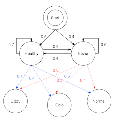
Consider a village where all villagers are either healthy or have a fever and only the village doctor can determine whether each has a fever. The doctor diagnoses fever by asking patients how they feel. The villagers may only answer that they feel normal, dizzy, or cold.
The doctor believes that the health condition of his patients operates as a discrete Markov chain. There are two states, “Healthy” and “Fever”, but the doctor cannot observe them directly; they are hidden from him. On each day, there is a certain chance that the patient will tell the doctor he is “normal”, “cold”, or “dizzy”, depending on their health condition.
It then provides the following parameters for the model:
model = HMM(
    hidden_sts=["healthy", "fever"],
    visible_sts=["normal", "cold", "dizzy"],
    trans_prob=[[0.7, 0.3], [0.4, 0.6]],
    obs_prob=[[0.5, 0.4, 0.1], [0.1, 0.3, 0.6]],
    ini_prob=[0.6, 0.4],
)
which is depicted in the diagram below:
We can run our algorithm with the sample observations:
obs = [0, 1, 2]
print(viterbi(model, obs))
To get
['healthy', 'healthy', 'fever']Conclusion
I learned about Viterbi’s Algorithm while studing HMMs in the context of speech recognition [3], which is my main topic of study this year.
The Wikipedia entry for this subject [1] is very good, so I was able to base my post entired off that. I found that the algorithm itself is not very complicated.
Related Posts
- Probabilistic Graphical Model Lecture Notes - Week 1. I’ve learned about HMMs a long time ago, and forgot most of it. It might be that I even learned about Viterbi’s algorithm at some point too. I’vew revisited and translated this post from my old blog in Portuguese.
