kuniga.me > NP-Incompleteness > Probabilistic Graphical Model Lecture Notes - Week 1
Probabilistic Graphical Model Lecture Notes - Week 1
18 Mar 2012
Tomorrow the Probabilistic Graphical Models (PGM) classes will begin. I will use the blog to record and organize my notes about the course.
According to the calendar there will be 10 weeks of classes, with theoretical and practical exercises, in addition to a final exam in early June.
As the recommendation is to dedicate 10 to 15 hours per week to study and I will probably only be able to study on weekends, I decided not to take the natural language processing course.
As the material for the first week is already available, I decided to go ahead.
Review
In the Introduction and Overview video series, the PGM concept and its applications are presented and basic probability concepts such as probability distribution functions, random variables, conditional probability are reviewed.
They are introduced definitions I did not know: factors, which are functions that take as input all combinations of the values of a set of random variables and return a scalar. This set of random variables is called scope.
We can think of factors as being tables. This makes it easier to understand the definition of the three operations presented on factors: product of factors, marginalization of factors and reduction of factors.
The product of two factors $A$ and $B$ is a factor $C$ whose scope is the union of the scopes of $A$ and $B$. The value returned by $C$ for a given input $i$ is given by multiplying the values returned by $A$ and $B$ for the inputs that are subsets of $i$.
The marginalization of a factor $A$ consists in generating a factor $A’$ with a subset of the scope of $A$. The value of an input $i’$ for $A’$ is given by adding the values of the inputs of $A$ of which $i’$ is a subset.
The reduction of a factor $A$ is a factor $A’$ with the value of some of the variables of the domain of $A$ fixed. The value of the input $i’$ for $A’$ corresponds to the value obtained from an input of $A$ corresponding to $i’$ plus the fixed values. It looks like a generalization of the conditional probability distribution.
Bayesian Networks
A Bayesian network is a directed acyclic graph (DAG). The vertices are the random variables and there is an edge $(u, v)$ if the random variable $v$ depends on $u$. Associated with each vertex we have a conditional probability distribution (CPD).
Chain rule for Bayesian networks. The chain rule is used to calculate the joint probability distribution, that is, a probability distribution considering all random variables in the network. Basically what the rule says is that this distribution can be obtained by multiplying the CPD’s using product factors.
If a distribution $P$ is obtained by multiplying the CPD’s of the vertices of a Bayesian network $G$, we say that $P$ factorizes $G$.
Note that given the joint probability distribution, we can determine the probability of each node via marginalization.
Patterns of Reasoning
Reasoning occurs when we observe (that is, fix the value of) a random variable $X$ and this affects the probability distribution of another variable $Y$. In a Bayesian network, we can classify inferences according to the relationship between variables $X$ and $Y$ in the graph.
- Causal Reasoning. is when the observed variable $X$ is the ancestor of variable $Y$.
- Evidential Reasoning. is when the observed variable $X$ is a descendant of variable $Y$.
- Intercausal Reasoning. is when the variables $X$ and $Y$ are not connected by a directed path.
Flow of influence
We say that there is a flow of influence from a variable $X$ to $Y$, if the observation of $X$ influences the probability distribution of $Y$. This flow also depends on which other variables in the network besides $X$ are observed. Then we refer to the evidence set as a set of network variables observed and we will call $Z$.
The influence of flow is represented by a path (not necessarily directed) in the graph, which is called the active trail. Let $X$, $W$ and $Y$ be variables corresponding to consecutive vertices in a path. The possible relationships between them are:
\[\begin{aligned} 1. \quad X \rightarrow W \rightarrow Y\\ 2. \quad X \leftarrow W \leftarrow Y\\ 3. \quad X \leftarrow W \rightarrow Y\\ 4. \quad X \rightarrow W \leftarrow Y \end{aligned}\]We will present the conditions in which there is a flow through $X$, $W$ and $Y$. For cases 1, 2 and 3, we have flow passage if and only if $W$ is not in $Z$. Intuitively, if $W$ is observed, it will “overtake” the influence from then on.
The most counterintuitive case is case 4, which is known as a V-structure. In general, if we know something about $X$, it doesn’t affect our knowledge about Y. However, if we know something about $W$, knowledge about $X$, it can affect knowledge about $Y$!
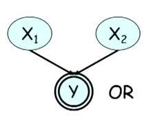
A good example is given at the end of the class Reasoning Patterns. The structure of Figure 1 is given, where $y = x_1 \mid x_2$. If we know the value of $y$, knowing the value of $x_1$ will change the probability of the value of $x_2$.
Thus the rule for case 4 is that either $W$ or any of its ancestors be $Z$. Finally, a path whose triplets of consecutive vertices respect the flow conditions, is an active path.
Independence
Conditional independence. When two random variables $X$ and $Y$ are independent for a distribution $P$, we say that P satisfies $X$ independent of $Y$, or that $P \models X \ perp Y$. The independence between $X$ and $Y$ given the observation of a variable $Z$ is represented by $(X \ perp Y \mid Z)$ and characterizes the conditional independence.
d-separation. In a Bayesian network G, if there is no active path between $X$ and $Y$ given a set of evidence $Z$, we say that there is a d-separation between $X$ and $Y$ given $Z$ in $G$, or more succinctly $d \mbox{-} sep_G (X, Y \mid Z)$.
Independence map. Let $I(G)$ be the set of conditional independence $(X, Y \mid Z)$ corresponding to d-separations of $G$, for all $X$, $Y$ and $Z$. If $P$ satisfies all indpendencies in $I(G)$, we say that $G$ is a map of $P$.
Given these definitions, we have the following theorem:
Theorem. $G$ is a map of independences for $P$ if, and only if, $P$ is a factorization over $G$.
With this theorem, we have two ways of seeing a Bayesian network: as factors (CPD’s of the vertices) of a distribution $P$ or as a set of independences that $P$ must satisfy.
Naive Bayes
A special class of Bayesian networks is the Naive Bayes, in which we have a node with several descendants, as shown in Figure 2.
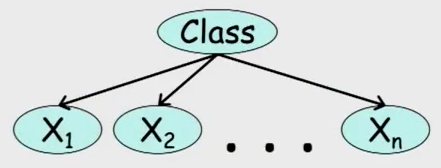
This structure is used for simple cases of classification. Child nodes are traits and the root is a random variable corresponding to the class. Thus, given an observation of the traits, one wants to know which class is most likely.
There are two common types of naive Bayesian classifiers, that of Bernoulli, where the traits assume a binary value and the multinomial where they can assume multiple values.
Note that this model implies independence between the traits given the class. This assumption can be very simplistic if the traits of the problem are highly correlated.
Template Models
Template Models aim to abstract structures that are repeated. This makes the model more compact and allows reuse in problems with similar structures.
Time Models
There are problems that must be modeled considering the passage of time. In general, we discretize time in pieces of fixed size and create random variables associated with each piece. In this case, the variable is usually represented by $X^{(t)} $ and a set of variables corresponding to an interval $t$ to $t’$ by: $X^{(t: t’)} = {X^{(t)}, \cdots, X^{(t’)}}$.
To simplify temporal models, we can make the following assumptions:
Markov Process. says that a variable of time $t$ depends only on time $t-1$, or in mathematical terms: $(X^{(t + 1)} \perp X^{(0: t-1)} \mid X^{(t)})$.
Invariance with respect to time. which assumes that the conditional probability distributions $P(X^{(t + 1)} \mid X^{(t)})$ are the same for all $t$.
2TBN (2-time-slice Bayesian Network) is a transition model between two time fragments. It defines a piece of Bayesian network representing the transition from a set of variables $X_1, \cdots X_n$ to another $X’_1, \cdots X’_n$ in the next instant of time. In this model, only the second set of variables has CPD and this model defines a joint conditional probability distribution for $X’_1, \cdots X’_n$.
Dynamic Bayesian Network dynamics. or DBN is a network that is the initial state and a 2TBN representing temporal transition. The expansion of this network, that is, the replication of the 2TBN for the subsequent moments of time, forms the ground bayesian network.
Hidden Markov Model
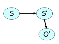
Also known as HMM is a type of DBN that uses a simplified version of the 2TBN in which we have only one variable $S$ that changes over time and an internal observation variable, as shown in Figure 3.
In addition, the possibilities for transition from one state to another in $S$ are limited. In the example in Figure 4, we cannot go from the $s_1$ state to the $s_3$ or $s_4$ states.
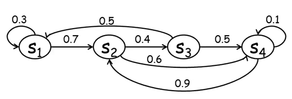
Plate models
Is a model that aims to factor parts common to several elements. The factored part can be a CPD common to all nodes or even a variable that is connected to several others, for example the difficulty of a course being linked to all students of that course.
The factored part is represented outside the plate and the objects that are repeated stay inside. The plate itself is drawn through a rectangle. It is possible to nest and also to overlap plates.
A template variable is defined as a set of random variables sharing a certain property. A limitation of this model is that the parents of a template variable that includes a $U$ set of variables, can only include a subset of $U$.
References
- [1] Coursera: Probabilistic Graphical Models 1: Representation
Notes
This is a review and translation done in 2021 of my original post in Portuguese: Probabilistic Graphical Models – Semana 1
