kuniga.me > NP-Incompleteness > Network Matrices
Network Matrices
30 Jun 2013
Introduction
In this post we’re going to write about a special case of the \(\{0, \pm 1\}\) matrix, which is called network matrix. They play an important role in our study of totally unimodular matrices.
We’ll first define a network matrix and provide an example. We’ll later show some properties and then describe a polynomial-time algorithm to recognize network matrices.
Definition
Network matrices were first defined by William Tutte (1965) [1]. The definition is the following:
Let \(D = (V, A)\) be a directed graph and \(T = (V, A_0)\) be a directed tree on the vertex set \(V\). Let \(M\) be the matrix \(A_0 \times A\)-matrix defined by \(a = (v, w) \in A\) and \(a' \in A_0\).
\[M_{a',a} = \left\{ \begin{array}{ll} +1 & \mbox{if the path } v\mbox{-}w \in T \mbox{ passes through}\\ & a \mbox{ in the same direction.}\\ -1 & \mbox{if the path } v\mbox{-}w \in T \mbox{ passes through}\\ & a \mbox{ in the opposite direction}.\\ 0 & \mbox{if does not pass through } a \mbox{ at all.} \end{array} \right.\]Matrices with this structure are called network matrices.
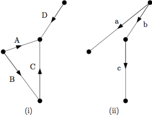
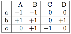
Example. In Figure 1 we see a sample digraph \(G(V,A)\) and a given directed tree \(T\) on the vertex set \(V\). The corresponding network matrix \(M\) represented by \(G\) and \(T\) is given on Table 1.

For each arc \((u,v) \in A\), we have a column in \(M\) representing the path from \(u\) to \(v\) in T. The signs indicate the direction of the edges in the path.

Properties
Let \(M\) be a network matrix, represented by the digraph \(G\) and the directed tree \(T\).
1) Multiplying a row of \(M\) by -1 is equivalent to inverting the direction of the corresponding edge in \(T\).
2) Multiplying a column of \(M\) by -1 is the same as inverting the direction of the corresponding edge in \(G\).
3) Deleting a row of \(M\) corresponding to edge \((i, j)\) of \(T\), is the same as shrinking vertex \(i\) and \(j\) into a single vertex.
4) Deleting a column of \(M\) is equivalent to removing the corresponding edge from \(G\).
Combining properties (3) and (4), we have that:
5) A submatrix of a network matrix is a network matrix as well.
The following theorem is the most important property about Network Matrices, that we’ll explore in the forthcoming posts about Integer Programming Theory:
Theorem 1. Networks matrices are Totally Unimodular.
Recognizing Network Matrices
There is a polynomial-time algorithm for deciding whether a matrix \(M\) is a network matrix. Without loss of generality we restrict ourselves to \(\{0, \pm 1\}\) matrices, since all network matrices are of this type and we can easily find out whether a matrix has such property.
We now divide it in two cases. Case 1: for all columns of \(M\), it has at most two non-zero entries; Case 2: the remaining types, that is, \(M\) has at least one column with three or more non-zero entries.
Case 1. Let’s describe the algorithm for the first case. Let M be a \(m \times n\), \(\{0,\pm 1\}\) matrix with at most 2 non-zero entries.
If \(M\) has, for each column, at most one entry 1 and at most one entry -1, we can show it’s a network matrix by constructing a digraph \(G\) and a tree \(T\) such that their corresponding network matrix is \(M\). We first build a direct star \(T\) with m vertices and with all edges pointing towards the center vertex \(v^*\). We now build the digraph \(G\) with the same vertex set. For each column in \(M\) that has an entry +1 and -1 for rows \((u,v^*)\) and \((w,v^*)\) we add an edge \((u,w)\). For columns having a single entry for row \((u, v^*)\), we add the \((u,v^*)\) to \(G\) if it’s +1 or \((v^*,u)\) if it’s -1.
The problem is that even in the restrictive Case 1, we may have both entries with the same signal. From property (1) though, we can multiply some rows by -1 and try to reach the case above. The question is then: can we split the rows into sets \(R_1\) and \(R_2\), in such a way that if we multiply rows in \(R_2\) by -1, we have at most one entry +1 and at most one entry -1 for all columns?
This question can be answered by a neat reduction to problem of deciding wether a graph is bipartite. Let \(G_R\) be a graph with vertex set corresponding to each row of \(M\) plus some artificial vertices. We add an edge \((i, j)\) if the corresponding rows have the same signal for some column. We add edges \((i, v_{ij}^*)\) and \((j, v_{ij}^*)\) if the have different signs. We then try to split this graph into two partitions \(R_1\) and \(R_2\).
The idea is that if such a partitioning exists, vertex with different signs will be in the same partition because they share a common vertex and vertex with the same signs must be on different partitions. If we now multiply all rows in \(R_2\) by -1, we’ll have our property.
Conversely, if no partition exists, it’s possible to show (see Example 1, from this post) that such matrix is not TU. Since by Theorem 1 all network matrices are TU, we conclude that this matrix is also not a network matrix. Summarizing we have that
Observation 1. The matrix \(M\) from the Case 1 is a network matrix if and only if its graph \(G_R\) define as above is bipartite.
Case 2. Now let’s concentrate on the more general case, where the matrix has at least one column with 3 or more non-zero entries.
For each row i of \(M\), we define a graph \(G_i\) with vertex set \(\{1, \cdots, m\} \setminus \{i\}\). There’s an edge between \(j\) and \(k\) if exists any column in M such that it has non-zero entries for j and k, but 0 for i. We have the following observation:
Observation 2. If \(M\) is a network matrix, there exists a row \(i\) for which \(G_i\) is disconnected.
The basic idea in understanding this observation is that since there is at least one column in \(M\) with three non-entries, there must be a path in T that connects two vertices in \(G\) with length at least 3. There is some edge i from the middle of this path that is not the first nor the last edge, henceforth denoted as \(j\) and \(k\). If we remove this edge, we will split it into two components. It’s then easy to see that any path in the tree that has \(j\) and \(k\) needs to go through \(i\). In turn, this means that there is no edge between the corresponding vertices in \(G_i\).
From Observation 2, we can conclude that if a given matrix has \(G_i\) for all possible columns \(i\), then \(M\) is not a network matrix.
So we can now suppose our candidate matrix has a disconnected \(G_1\) (we can assume \(i = 1\) without loss of generality. Let \(C_1, \cdots, C_p\) be the connected components of \(G_1\).
We define
-
\(W :=\) as the set of column indexes for which the first row of M has non-zero entries;
-
\(W_i := W \cap\) the set of column indexes for which the \(i\)-th row of \(M\) has non-zero entries;
- \[U_k := \bigcup \{W_i \mid i\in C_k\}\]
Now, we build a graph \(H\) with vertex set \(\{C_1, \cdots, C_p\}\), with an edge \((C_k, C_\ell)\) if the following conditions are met:
-
\(\exists i \in C_k: U_\ell \not \subseteq W_i\) and \(U_\ell \cap W_i \neq \emptyset\)
-
\(\exists j \in C_\ell: U_k \not \subseteq W_j\) and \(U_k \cap W_j \neq \emptyset\)
and let \(M_k\) be the submatrix formed by the rows of \(M\) corresponding to vertices in \(C_k\).
We now can state the following Theorem:
Theorem 2. M is a Network Matrix if and only if: \(H\) is bipartite and \(M_k\) is a network matrix for \(k=1, \cdots, p\).
Complexity
Theorem 3. The algorithm above to detect whether a given matrix \(M\) is a network matrix has polynomial-time complexity.
-
Check if has only entries in \(\{0, \pm 1\}\)
-
Test if has at most two non-zero entries for each column (Case 1 or Case 2)
-
Case 1: Construct the graph \(G_R\) and check whether it is bipartite.
-
Case 2: For each column i, construct graph \(G_i\) and check if it is not connected. In this case, we build the graph \(H\) and build each of the submatrices \(M_k\).
If we assume the matrix is \(m \times n\), (1) and (2) can be performed in linear size of the matrix, \(O(mn)\). We can construct \(G_R\) in \(O(mn)\) as well and test for bipartiteness in linear time on the number of vertices plus the edges of \(G_R\), which are both \(O(n + m)\), so (3) is bounded by \(O(mn)\) too.
For step (4), we need to generate the graph \(G_i\). Its edges are bounded by \(mn\) and we can decide it’s connected in linear time of its size. Doing this for all \(n\) columns we a total complexity of \(O(mn^2)\).
For the recursive complexity, we can relax our complexity for Steps 1 to 4 to be \(O(n^tm^t)\) for a fixed constant \(t \ge 2\). By induction, we assume our total complexity for a given level of the recursion is \(O(n^{t+1}m^t)\).
The matrix \(M_k\) has \(m_k\) rows and \(n\) columns, can be solved, by induction, in \(O(m_k^{t+1}n^t)\). Summing up all the complexities we have:
\(O(m^tn^t) + O(m_1^{t+1}n^t) + O(m_2^{t+1}n^t) + \cdots + O(m_p^{t+1}n^t)\) which is \(O(m^{t+1}n^t)\)
The base is when we do steps 1 to 4 without building any submatrices, which we saw it is \(O(m^tn^t)\).
Conclusion
The main points to be taken from this post is that network matrices are totally unimodular and that they can be recognized in polynomial-time.
We provided explanations about the two observations, but we left out the proofs of the Theorems 1 and 2, which are quite long and complicated, and thus out of the scope of the post. Nevertheless, they can be found on [1].
References
- [1] Theory of Linear and Integer Programming – A. Schrijver (Chapter 19)
