kuniga.me > NP-Incompleteness > Multi-valued functions
Multi-valued functions
15 Dec 2024
In particular, we'll formalize the notion of restricting the image of a multi-valued function to turn it into a single-valued one.
N-th Root
When we first learn about square roots of positive reals, we learn that it produces two values, a positive and negative, so for example, the square root of $9$ is both $3$ and $-3$. For the cubic root we don’t have to worry about the negatives, so we can usually claim that, for example, $27^{1/3} = 3$.
Then we learn about complex numbers and learn that the $n$-th root actually produces $n$ values. It just happens that for positive values and $n = 2$, it produces two complex numbers with zero imaginary part, but for $n = 3$ the other two values have non-zero imaginary parts.
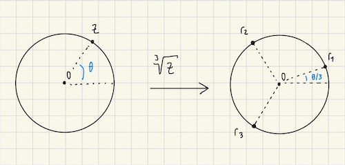
More generally, a complex number can be written in polar form as $z = \abs{z}e^{i\theta}$, where $\theta$ is the angle of $z$ with respect to the positive real axis. The $n$-root generates values of the form:
\[\abs{z}^{1/n} \exp\paren{i(\theta + 2k\pi)/n} \quad k = 0, \cdots, n-1\]Geometrically, we can interpret these as $n$ points in the circumference of a circle centered at the origin with radius $\abs{z}^{1/n}$, equally spaced and started with an offset $\theta / n$.
So the $n$-th root is a multi-valued function, which is not nice to work with. Is it possible to obtain a single-valued function from a multi-valued one?
One idea is to restrict the image to a subset in which only one value is allowed. For example, for the square root, we could restrict the image to only numbers that have non-negative real values. This would work well for complex numbers with non-zero real parts, since they have at least one of the roots in the positive $x$-axis.
It would not work for points on the $y$-axis (i.e. zero real part) because both its roots would be included. If we changed the image restriction to “only numbers that have positive” real parts, then both roots would be excluded. It can get complicated.
In the rest of this post, we’ll study a framework for restricting the image to obtain a single-valued function from a multi-valued one.
A Moving Point
The complex plane is a valueable tool to “visualize” complex numbers making them more intuitive. We typically consider points in a static way, like an image, but we could generalize it to a movie or animation.
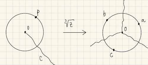
Let’s consider the function $f(z) = z^{1/3}$. As we’ve discussed, it maps each point onto $3$ others on the image. Let fix a point $p$ in the unit circle and name its images $a$, $b$ and $c$, like in Figure 2.
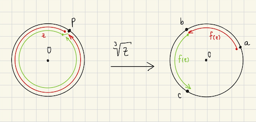
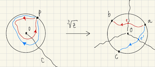
Now imagine we have a point $z$ at $p$ and we start moving it along the circumference shown in Figure 2, counter-clockwise. The point $z$ will have 3 images, but let’s arbitrarily focus on one of the images, say the one starting at $a$.
As we move $z$ with angular speed $\omega$, its image will move accordingly along the corresponding circumference, except that it will have angular speed $\omega / 3$.
Which means that once $z$ completes a full revolution (red path in Figure 2), it will be back at $p$, but its image will be $1/3$ of the way in, at $b$! If $z$ completes another revolution (green path in Figure 2), its reaches $c$ and on the third revolution of $z$ (not depicted in Figure 2) the image finally gets back to $a$.
Branch Point
Now, suppose $z$ doesn’t have to move along the circumference. It’s free to wander around the way it wants, as long as it comes back to $p$. As before, suppose we’re looking initially looking at the image $a$ of $p$. Can we tell in which of the images of $p$ will $z$ end up with once it’s back at $p$?
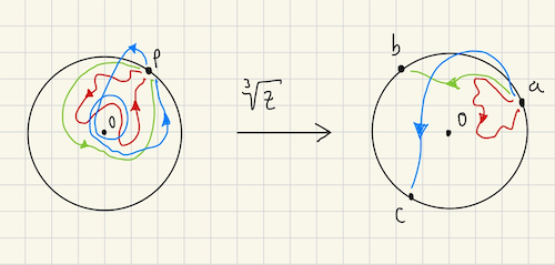
By considering some examples we’ll notice that it changes to a different image depending on whether it completes a revolution over the origin. For $z^{1/3}$, the origin is the point for which all three images coincide, a singularity.
Such a point (the origin in this case) is called the branch point.
Branch Cut
One way to avoid a function from generating multiple values when “moving a point around”, is to prevent it from encircling the branch point. One way to do this is to draw a line from the branch point to the infinity, and remove points on that line from the domain, for example the curve $C$ in Figure 4 (left).
This line is called the branch cut. If the branch point is the origin, a common choice for the branch cut is the non-positive real axis.
Branches
If we exclude the points on the branch cut $C$, we can partition the image into regions defined as follows: Let $\Omega$ be the original domain of $f(z)$. Let $z$ and $w$ be distinct points in $\Omega \setminus C$. Then points $f(a)$ and $f(b)$ belong to the same region if there’s a path from $z$ to $w$ in $\Omega \setminus C$.
For $f(z) = z^{1/3}$ we could have something like:
Now if we add the points of the branch cut back, they form the boundary between the regions.
Let’s consider the example of $z$ starting from $p$ and going around the origin once. Suppose it starts at $f(p) = a$. It will eventually cross the branch cut at some point $e$ which corresponds to crossing between regions and then eventually reach $f(p) = b$.
To which region do the points on the border (i.e the image of $C$) belong to? We can arbitrarily assign it to one of the regions but we need to be careful: a region is “flanked” by two of the images of the branch cut, so if we assign one copy to a region, the other copy must go to the other region. Because the idea is to have each region have exactly one copy of the image of a point in the domain.
A simple way to acheieve that is to say that if $z$ crosses the border in the counter-clockwise direction (with respect to the branch point), that border belongs to the region it is in. Otherwise it belongs to another region. Figure 5 illustrates this.
With this setup, for each of these regions, we can find a single-valued function from $\Omega \setminus C$ onto that region. This function is called a branch of $f(z)$.
Principal Branch
Supposing we choose the negative real axis as the branch cut, one simple way to prevent a path from crossing it is to restrict the domain to points with arguments within $-\pi \lt \theta \le \pi$. This is defined as the principal value of the argument.
For this domain, for each multi-valued function there’s usually a branch that is used by default and it’s denoted as the principal branch. For example, for $f(z) = z^{1/3}$, the principal branch is defined to be $f(z) = \abs{z}^{1/3} e^{i\theta/3}$ and can be denoted by square brakets: $[z^{1/3}]$.
The other two branches would be $f(z) = \abs{z}^{1/3} e^{i(\theta + 2\pi)/3}$ and $f(z) = \abs{z}^{1/3} e^{i(\theta + 4\pi)/3}$.
Conclusion
I’ve seen branch points and branch cuts mentioned in Alfhor’s Complex Analysis book that I’ve been studying. I skimmed through it in one of the early chapters but found I didn’t fully grasp it in a discussion in a later point.
I decided to buy Tristan Needham’s Visual Complex Analysis book and his explanation on this topic is superb and intuitive. This post is based off his book.
I now regret having started with Alfhor’s book having peeked at Tristan Needham’s. The problem is that Visual Complex Analysis covers the topics in a completely different order, so I’m not eager to start over and try to map topics that I’ve already seen. I will however keep using Needham’s book as a complement.
References
- [1] Visual Complex Analysis, Tristan Needham.
