kuniga.me > NP-Incompleteness > Levinson Recursion

Levinson Recursion

20 Feb 2021

Norman Levinson was an American mathematician, son of Russian Jewish immigrants and grew up poor. He eventually enrolled at MIT and majored in Electrical Engineering but switched to Mathematics during his PhD in no small part due to Norbert Wiener.

Levinson spent two years at the Institute for Advanced Study at Princeton where we has supervised by von Neumann. During the Great Depression, Levinson applied to a position at MIT and was initially refused, likely due to anti-semitic discrimination. The famous British mathematician G. H. Hardy intervened and is reported to have said to the university’s provost, Vannevar Bush:

Tell me, Mr Bush, do you think you’re running an engineering school or a theological seminary? Is this the Massachusetts Institute of Theology? If it isn’t, why not hire Levinson.

Levinson got the job in 1937 but almost lost it during the McCarthy era due to an initial association with the American Communist Party. Levinson passed away in 1975 [1].

In this post we’ll discuss the Levinson Recursion algorithm, also known as Levinson–Durbin recursion, which can be used to solve the equation $A x = y$ more efficiently if $A$ obeys some specific properties.

Toeplitz Matrix

A Toeplitz matrix or diagonal-constant matrix is a matrix where all the elements in the top-left to bottom-right diagonals are the same.

In other words, let $T$ be matrix with elements $t_{ij}$. $A$ is a Toeplitz iff $t_{ij} = t_{i-1, j - 1}$ for all $i > 1$ and $j > 1$.

A Toeplitz matrix is not necessarily square. An example:

For this post, we’ll assume $T$ is square and we’ll represent its indices generically as:

Submatrices along the diagonal

Let $T$ be a $n \times n$ matrix, consider a submatrix of size $m$, $T^m$ of $T$ with $m < n$, aligned on their first element. More precisely, $t_{ij}^{m} = t_{ij}$ for $1 \le i, j \le m$.

It’s easy to see that if $T$ is a Toeplitz matriz, so is $T^m$.

Furthermore, suppose we have another submatrix $U^m$ but with the first element of $U^m$ aligned on $t_{2,2}$, that is $u_{ij}^{m} = t_{i + 1, j + 1}$ for $1 \le i, j \le m$. If $T$ is a Toeplitz matrix, then $U^m = T^m$.

In fact, all submatrices of a given size $m$ are the same if their first elements are aligned on the diagonal of $T$. We can get an intuition from the following example:

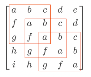
This property will be important later, so let’s keep it in mind.

Levinson Recursion

Given a $n \times n$ Toeplitz matrix and a vector $y$, the Levinson recursion can solve equation $Tx = y$ for $x$ in $O(n^2)$ by using intermediate vectors called forward and backward vectors.

Forward and Backward vectors

Let $e_i$ be the column vector with all zeroes, except in row $i$ which is 1. We define $f^i$ such that

and $b^i$ such that

We can compute $f^i$ and $b^i$ recursively, that is, we assume we know $f^k$ and $b^k$ for $k < n$ and show how to obtain $f^i$ and $b^i$.

We start by appending a 0 to $f^{i - 1}$, which we’ll call $\hat f^i$. What happens if we multiply $T^i$ by it?

To compute this, we can define in terms of $T^{i-1}$:

We’ll end up with a $i \times 1$ column vector, where the first $i - 1$ entries are from

The last entry, a scalar, will come from

Which we’ll denote as $\epsilon_f^i$, thus

So we almost got $e_1$! The only extraneous bit is $\epsilon_f^i$. The idea now is to try to eliminate that. Before that, we can use the same idea to get an analogous result for $\hat b^i$, that is:

Note how we’re using the property discussed in Submatrices along the diagonal so that

Without this property this recurrence wouldn’t work. We also assume that:

We will now show that a linear combination of $\hat f^i$ and $\hat b^i$ can yield the desired results, that is

for scalars \(\alpha_f^i, \beta_f^i, \alpha_f^i, \beta_f^i\). Since $T^i f^i = e_1$:

This will gives us a set of equations, but only the first and last entries are non trivial:

Since $T^i b^i = e_i$:

Noting that $\epsilon_f^i$ and $\epsilon_b^i$ are constants, we have 4 unknowns and 4 equations (4-7), so we can obtain:

Using (2) and (3) we can obtain $f^i$ and $b^i$.

It remains to define the base case. We need to find $f^1$ such that $T^1 f^1 = [t_0] f^1 = [1]$, hence $f^1 = [\frac{1}{t_0}]$. The same applies to $b^1$.

Using the backward vector

We can solve $T x = y$ recursively, that is if we know how to solve $T^k x^k = y^k$ for $k < i$ we can solve for $T^i x^i = y^i$.

Let’s define $\hat x^i$ as the column vector obtained by appending 0 to $x^{i-1}$. Then

Let $\epsilon^i_x = \sum_{j = 1}^{i - 1} t_{i - j} x_i$. Then

If we can replace that $\epsilon^i_x$ with $y_i$ we’d be able to obtain $x^i$! Suppose we can modify $\hat x^i$ by adding $\delta^i$ to obtain $x^i$:

So

Since $e^i = T^i b^b$, we have $T^i \delta^i = (y_i - \epsilon^i_x) b^i$. Wrapping up,

\((8) \quad x^i = \hat x^i + (y_i - \epsilon^i_x) b^i = \begin{bmatrix} x^{i-1} \\ 0 \end{bmatrix} + (y_i - \epsilon^i_x) b^i\).

It remains to work out the base case, $T^1 x^1 = [t_0] x^1 = [y_1]$, so $x^1 = [y_1 / t_0]$.

The solution we’re seeking is $x = x^i$.

Time Complexity

In the forward and backward vectors step, we need $O(n)$ to operations to compute $\epsilon_f^i$ and $\epsilon_b^i$, at each iteration $n$, for a total of $O(n^2)$.

During the final step, we need $O(n)$ to compute $\epsilon_x^i$ and also $(8)$ at each iteration $n$, for a total of $O(n^2)$.

So overall the algorithm has $O(n^2)$ complexity, compared to $O(n^3)$ from a Gaussian elimination for general matrices.

Python Implementation

We now provide an implementation of these ideas using Python.

def levinson(mat, y):

    n = len(mat)

    t_0 = mat[0][0]
    # forward vector f^i
    f = np.array([1.0/t_0])
    # backward vector b^i
    b = np.array([1.0/t_0])
    # partial solution x^i
    x = np.array([y[0]/t_0])

    for i in range(1, n):
        last_row = mat[i, 0 : i + 1]
        f2 = np.append(f, 0)
        eps_f = np.dot(last_row, f2)

        first_row = mat[0, 0 : i + 1]
        b2 = np.insert(b, 0, 0)
        eps_b = np.dot(first_row, b2)

        # Common denominator to all alphas and betas
        denom = 1. - eps_f * eps_b

        # Compute f^i from b^(n-1) and f^(n-1)
        alpha_f = 1. / denom
        beta_f = -eps_f / denom
        f = alpha_f * f2 + beta_f * b2

        # Compute b^i from b^(n-1) and f^(n-1)
        alpha_b = -eps_b / denom
        beta_b = 1 / denom
        b = alpha_b * f2 + beta_b * b2

        # Compute x^i from b^i
        x2 = np.append(x, 0)
        eps_x = np.dot(last_row, x2)
        x = x2 + (y[i] - eps_x) * b

    return x

The full code is on Github.

Let’s make some observations on the code. First, we use numpy, especially it’s dot function which performs a dot product between two vectors of the same size. We also leverage the overloaded operators with numpy.arrays which behave more like in linear algebra.

For example, adding two numpy.arrays does element-wise sum:

np.array([1, 2]) + np.array([3, 4]) # np.array([5, 6])

while Python lists concatenates. Another example is multiplying by a scalar:

np.array([1, 2]) * 10 # np.array([10, 20])

Note that while we describe the computation of $b^i$ and $f^i$ vs. $x^i$ separately, in code we compute them at the same time because $x^i$ needs $b^i$.

Conclusion

I ran into this algorithm while studying signal processing, in particular Linear Predictive Coding which I plan to write about later.

The idea is pretty clever and I was wondering how could one have thought of it. One possible way was to assume some induction property and try to jump from a solution of $k - 1$ to $k$. This is a similar line of thinking we use when trying to see if a problem can be solved by dynamic programming for example.

By playing around with extending the solution, we could have tried appending a 0 and observing it almost looks like what we want, except that we need to “override” the last element. From there, we can reduce to a simpler problem which is to solve $Tx = e_i$, which is exactly the backward vector equation.

For solving $Tb = e_i$ recursively, maybe we would realize that it’s simpler to preprend instead of appending a 0, since for $e_i$ and $i > 1$, the first position will be always zero which is easier to work with. Now we got that $\epsilon_b$ we need to eliminate, which is now in the first position, so we get to $Tf = e_1$, that is, the forward vector.

We then have a “cyclic dependency” since to solve $Tf = e_1$ we would need $Tb = e_i$. But maybe we can resolve that by using them at the same time? Because we’re working with $e_i$ and $e_1$ we might think of an orthogonal basis spanning a vector space via linear combination equations like we did with equations (4-7).

This exercise of trying to find how an algorithm came to be was helpful to me. We often only see the final polished result of an idea but the intermediate steps are often more intuitive and more likely to be reused for solving future problems.

Related Posts

Quantum Fourier Transform - The Levinson algorithm uses a technique of “manipulating” a solution with curgical precision by leveraging the $e_i$ vector, which when multiplied by a scalar can be added to the solution and only modify a single element. This reminded me of the Quantum Fourier Transform circuit where we use the $CR_2(\psi, j_n)$ gate to “inject” a bit.

References

• [1] MacTutor - Norman Levinson
• [2] Wikipedia - Levinson Recursion

Source code | RSS feed | Tags: linear algebra