kuniga.me > NP-Incompleteness > L-BFGS
L-BFGS
04 Sep 2020
BFGS stands for Broyden–Fletcher–Goldfarb–Shanno algorithm [1] and it’s a non-linear numerical optimization method. L-BFGS means Low Memory BFGS and is a variant of the original algorithm that uses less memory [2]. The problem it’s aiming to solve is to mimize a given function \(f: R^d \rightarrow R\) (this is applicable to a maximization problem - we just need to solve for \(-f\)).
In this post we’ll cover 5 topics: Taylor Expansion, Newton’s method, QuasiNewton methods, BFGS and L-BFGS. We then look back to see how all these fit together in the big picture.
Taylor Expansion
The Taylor expansion [3] is a way to approximate a function for a given value if we know how to compute it and its derivatives around that point.
The function might be hard to compute at a given point but if we know how to compute derivatives around that point we can get a good approximation.
The geometric intuition in 2D is that our function is a curve \(y = f(x)\) and we want to compute \(f()\) for a given \(x'\). If we know how to compute \(f'()\) for a given \(a\) that is sufficiently close to \(x'\), then \(f'(a)\) represents the coeficient of a line, the tangent of \(f()\) at \(a\), so \(f(x') \sim f(a) + f'(a) (x' - a)\).
Depending on the distance of \(x'\) and \(a\) and the “curvature” of \(f()\), the approximation might be too off. The idea is to add higher degree polinomials so that the polinomial resembles \(f()\)’s shape better. Taylor expansion does exactly this though I lack the geometric intuition for these extra terms. Given \(f: R \rightarrow R\), its Taylor expansion is:
\[f(x) \sim f(a) + \frac{f'(a)}{1!} (x - a) + \frac{f^{''}(a)}{2!} (x - a)^2 + \frac{f^{'''}(a)}{3!} (x - a)^3 ...\]or in a compact form:
\[f(x) \sim \sum_{k=0}^{\infty} \frac{f^{(k)}(a)}{k!} (x - a)^k\]Where \(f^{(k)}\) is the \(k\)-th derivative of \(f()\), and assuming \(f^{(0)} = f\).
Example: sin(x)
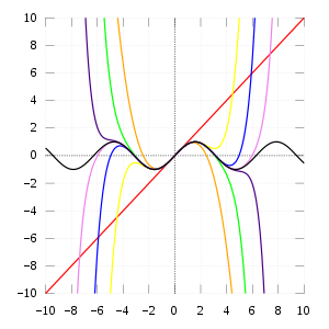
One interesting application of the Taylor Expansion is computing sin(x). We have that \(\frac{d(sin(x))}{dx} = cos(x)\) and \(\frac{d(cos(x))}{dx} = -sin(x)\), so according to Taylor:
\[sin(x) \sim sin(a) + \frac{cos(a)}{1!} (x - a) + \frac{-sin(a)}{2!} (x - a)^2 + \frac{-cos(a)}{3!} (x - a)^3 ...\]If we choose $a=0$, then we can use the knowledge that \(sin(0)=0\) and \(cos(0)=1\) and get
\[sin(x) \sim x - \frac{x^3}{3!} + \frac{x^5}{5!} ...\]Again, this is assuming \(x\) is around \(a=0\). This might not a good approximation for \(sin(1)\) for example.
Multi-variate
The Taylor expansion we defined assumes $x$ is a scalar. If we go back to our multi-dimensional function, \(f: R^d \rightarrow R\), we can define the expansion as:
\[f(x_1,..., x_d) \sim f(a_1, ..., a_d) + \sum_{j=1}^{d} \frac{\partial f(a_1, ..., a_d)}{\partial x_j} (x_j - a_j) +\] \[\quad\quad \frac{1}{2!} \sum_{j=1}^{d} \sum_{k=1}^{d} \frac{\partial^2 f(a_1, ..., a_d)}{\partial x_j \partial x_k} (x_j - a_j)(x_k - a_k) + ...\]As we can see, this notation is very verbose, so let’s use some common terminology/symbols from vectors. 1) Vector notation: \(\vec a = (a_1, ..., a_d)\). 2) The gradient defined as \(\nabla f(\vec x) = (\frac{\partial f(\vec x)}{\partial x_1}, ..., \frac{\partial f(\vec x)}{\partial x_d})\), so the sum
\[\sum_{j=1}^{d} \frac{\partial f(a_1, ..., a_d)}{\partial x_j} (x_j - a_j)\]can be re-written as:
\[(\vec x - \vec a)^T \nabla f(\vec x)\]Recalling that \(\vec u^T \vec v\) is the inner product of \(\vec u\) and \(\vec v\).
3) The Hessian matrix defined as:
\[\nabla^2 f(\vec x) = \begin{bmatrix} \frac{\partial^2 f}{\partial x_1^2} & \dots & \frac{\partial^2 f}{\partial x_1 \partial x_d} \\ \vdots & \ddots & \vdots \\ \frac{\partial^2 f}{\partial x_d \partial x_1} & \dots & \frac{\partial^2 f}{\partial x_d^2} \end{bmatrix}\]that is \(\nabla^2 f(\vec x)_{ij} = \frac{\partial^2 f}{\partial x_i \partial x_j}\) and we can show that this double summation:
\[\sum_{j=1}^{d} \sum_{k=1}^{d} \frac{\partial^2 f(a_1, ..., a_d)}{\partial x_j \partial x_k} (x_j - a_j)(x_k - a_k)\]can be rewritten as:
\[(\vec x - \vec a)^T \cdot \nabla^2 f(\vec x) \cdot (\vec x - \vec a)\]We included the \(\cdot\) just so it’s obvious where the multiplications are. To get a sense on why this identity is correct, we can look at \(d=2\):
\[\frac{\partial^2 f(a_1, a_1)}{\partial^2 x_1} (x_1 - a_1)(x_1 - a_1) + \frac{\partial^2 f(a_1, a_2)}{\partial x_1 \partial x_2} (x_1 - a_1)(x_2 - a_2) +\] \[\quad \frac{\partial^2 f(a_2, a_1)}{\partial x_2 \partial x_1} (x_2 - a_2)(x_1 - a_1) + \frac{\partial^2 f(a_2, a_2)}{\partial^2 x_2} (x_2 - a_2)(x_2 - a_2)\]equals to
\[\begin{bmatrix} x_1 - a_1 \\ x_2 - a_2 \end{bmatrix} \begin{bmatrix} \frac{\partial^2 f}{\partial x_1^2} & \frac{\partial^2 f}{\partial x_1 x_d} \\ \frac{\partial^2 f}{\partial x_2 \partial x_1} & \frac{\partial^2 f}{\partial x_2^2} \end{bmatrix} \begin{bmatrix} x_1 - a_1 & x_2 - a_2 \end{bmatrix}\]For a Taylor expansion of order two, which we’ll see next is of special interest to us, can be described more succinctly as:
\[(1) \quad f(\vec x) \sim f(\vec a) + (\vec x - \vec a)^T \nabla f(\vec x) + \frac{1}{2} (\vec x - \vec a)^T \nabla^2 f(\vec x) (\vec x - \vec a)\]Newton’s Method
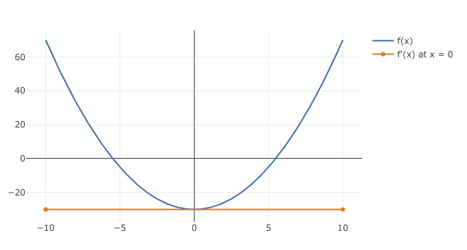
Newton’s Method [4, 5] can be used to optimize a function. At its core, it relies on the fact that we can find the minimum of a quadratic equation through it’s derivative. Let \(f: R \rightarrow R\) be a quadratic function, \(f(x) = ax^2 + bx + c\), with \(a > 0\) (otherwise the minimum value would be unbounded). In 2D the function \(f(x)\) looks like a parabola when plotted against x.
Drawing intuition from this 2D case above, the derivative can be seen as the rate of change for the curve at a given point x. It starts out as negative and becomes positive when the curve bounces back upwards, but because the curve is smooth, it has an inflection point where the rate of change is 0. This is also where the lowest value $f(x)$ takes and hence is our optimal value.
Mathematically, we can get the derivative of our second order polynomial as:
\[f'(x) = 2ax + b\]and find the \(x^*\) for which it’s 0:
\[2ax^* + b = 0\] \[(2) \quad x^* = -b/2a\]Now say we want to minimize an arbitrary function (which is not necessarily quadratic), \(f: R \rightarrow R\), which we’ll call \(f^*\).
Suppose we pick a value of \(x_0\) which we think is a good solution to \(f^*\). We might be able to improve this further by moving around \(x_0\), by some \(\Delta x\). Say our neighbor point is \(x = x_0 + \Delta x\).
We can now go back to our Taylor expansion of order 2 by replacing a with \(x_0\):
\[f(x) \sim f(x_0) + \frac{f'(x_0)}{1!} (x - x_0) + \frac{f^{''}(x_0)}{2!} (x - x_0)^2\]if we express this in terms of only \(x_0\) and \(\Delta x\) we get:
\[(3) \quad f(x) = f(x_0 + \Delta x) \sim f(x_0) + \frac{f'(x_0)}{1!} \Delta x + \frac{f^{''}(x_0)}{2!} (\Delta x)^2\]To mimimize $f(x)$ we can minimize the right hand side of that equation, which is a quadratic function on \(\Delta x\)! This means we can use (2) to find such \(\Delta x\).
In our expression above, \(a = \frac{f^{''}(x_0)}{2!}\) and \(b = \frac{f'(x_0)}{1!}\), so this yields:
\[\Delta x = -\frac{f'(x_0)}{f^{''}(x_0)}\]We can find the best neighbor \(x\) via:
\[x = x_0 -\frac{f'(x_0)}{f^{''}(x_0)}\]This expression can be used as recurrence to find smaller values of \(f(x)\) from an initial \(x_0\):
\[x_n = x_{n-1} -\frac{f'(x_{n-1})}{f^{''}(x_{n-1})}\]We can generalize it to higher dimensions, based on the general form of the Taylor expansion (1):
\[\vec x_n = \vec x_{n-1} - (\nabla^2 f(\vec x_{n-1}))^{-1} \nabla f(\vec x_{n-1})\]Recalling from matrix arithmetic, the way to “divide” a given \(d\)-dimension vector \(v\) by a \(d \times d\) matrix \(M\), is to find the “quotient” \(q\) such that \(v = qM\). We can multiply both sides by \(M^-1\) and get \(vM^{-1} = q(MM^{-1}) = qI = q\), which is what we’re doing with \(\nabla f(\vec x_{n-1})\) and \(\nabla^2 f(\vec x_{n-1})\) above.
The main problem of this method is the cost of computing the inverse of the Hessian matrix on every step. The simplest way to do it (Gauss–Jordan elimination) is \(O(n^3)\), while the best known algorithm is \(O(n^{2.373})\).
We’ll now cover a class of methods aiming to address this bottleneck.
QuasiNewton Methods
The QuasiNewton Methods [6] are a class of methods that avoids computing the inverse of the Hessian by using an approximation matrix, which we’ll denote \(B_n\), whose inverse can be more efficiently computed from the inverse of a previous iteration (\(B_{n-1}\)).
One of the common properties methods in this class have is that they satisfy the secant condition. Let’s see what this means. Recall that the second-order Taylor expansion for \(x \in R\) (3), but now renaming \(x\) to \(x_{n+1}\) and \(x_0\) to \(x_n\), and \(\Delta x\) renamed to \(y_n\) to make it clear that \(\Delta x\) is different on each iteration:
\[f(x_{n+1}) = f(x_n) + \frac{f'(x_n)}{1!} y_n + \frac{f^{''}(x_n)}{2!} y_n^2\]Which is a quadratic function on $y_n$. If we derive on $y_n$ we get the direction of the function:
\[\frac{df(x_{n+1})}{d y_n} = f'(x_n) + f^{''}(x_n) y_n\]The multi-dimensional version is:
\[(4) \quad \nabla f(\vec x_{n+1}) = \nabla f(\vec x_n) + \nabla^2 f(\vec x_n) \vec y_n\]The secant condition states that the approximation matrix must satisfy (4), that is:
\[\nabla f(\vec x_{n+1}) = \nabla f(\vec x_n) + B_n \vec y_n\]If we define \(\vec s_n = \nabla f(\vec x_{n+1}) - \nabla f(\vec x_n)\), the equation can be more succintly expressed as:
\[(5) B_n \vec y_n = \vec s_n\]Also a further constraint can be added that \(B\) is symmetric [6]. Given these constraints, the different methods define $B$ as the optimal solution to this objective function:
\[B_{n+1} = argmin_{B} \, \| B - B_k \|\]According to Wikipedia:
The various quasi-Newton methods differ in their choice of the solution to the secant equation.
Where $| . |$ is a matrix norm, and \(\| B - B_k \|\) can be thought out as distance between \(B\) and \(B_k\). Thus the optimization problem we’re trying to solve is to find a matrix that satisfy the secant condition and is as close (where “distance” is defined by the norm) as possible to the current approximation \(B_k\).
Once we have an approximate of the Hessian, we can use to compute the direction in the Newton method via (5):
\[B_n \vec y_n = \vec s_n\]Multiplying by \(B_n^{-1}\):
\[\vec y_n = B_n^{-1} \vec s_n\]Since \(\vec x_{n+1} - \vec x_n = \vec y_n\):
\[\vec x_{n+1} = \vec x_n + B_n^{-1} \vec s_n\]Meaning that once we have \(B_n^{-1}\) we only need to compute \(\nabla f(\vec x_{n + 1})\) to obtain the next $\vec x_{n+1}$.
The BFGS Method
The BFGS method uses what is called the weighted Frobenius norm [7, 8] and defined as:
\[\| M \|_W = \| W^{1/2} M W^{1/2} \|_F\]For some positive definite matrix that satisfies \(W \vec s_n = \vec y_n\) (note how this is the reverse of (5)). And the Frobenius norm of a matrix $M$, $| M |_F$, is the square root of the square of all its elements.
The solution to this minimization problem is
\[(6) \quad B^{-1}_{n+1} = (I - \rho_n s_n y_n^T) B^{-1}_n (I - \rho_n y_n s_n^T) + \rho_n s_n s_n^T\]where \(\rho_n = (y_n^T s_n)^{-1}\), and \(\vec y_n = B_n^{-1} \vec s_n\). We’ll have \(B^{-1}_n\) from the previous iteration and we can compute \(\vec s_n\) from \(\nabla f(\vec x_{n}) - \nabla f(\vec x_{n - 1})\).
The L-BFGS Method
We just saw we can use QuasiNewton methods to avoid the cost of inverting it, but we still need to store \(B_n\) in memory, which has size \(O(d^2)\) ans might be an issue if \(d\) is very large.
The Low Memory BFGS avoids the problem by not working with \(B\) directly. It computes \(B_n^{-1} \vec s_n\) (which uses only \(O(d)\) memory) without ever holding \(B_n\) in memory. It’s an interactive procedure to compute \(B_n^{-1}\) from \(B_0^{-1}\). Nocedal [9] defines the following interactive algorithm (I don’t understand how this was derived from (6) but he mentions it was originally proposed by [10], which unfortunately I don’t have access to):
For a given $n \in {0, \dotsc, N}$, where $N$ is the number of iterations:
- $q_n \leftarrow s_n$
- $\mbox{for} \, i = n - 1, \dotsc, 0:$
- $\quad\alpha_i \leftarrow \rho_i s_i^T q_{i+1}$
- $\quad q_i \leftarrow q_{i + 1} - \alpha_i y_i$
- $r_0 \leftarrow B_0^{-1} q_0$
- $\mbox{for} \, i = 0, \dotsc, n - 1:$
- $\quad \beta_i \leftarrow \rho_i y_i^T r_i$
- $\quad r_{i+1} \leftarrow r_{i} + s_j (\alpha_i - \beta_i)$
- $\mbox{return} \, r_n$
Note that $\alpha$ is the only variable shared among the two-loops, so it has to be stored. In addition, we need to keep $s_i$ and $y_i$ from all the previous $n$ iterations, so their size amounts to \(O(dN)\), where $N$ can be very large depending on convergence conditions. The proposal of L-BFGS is to define $m \lt \lt N$ and only work with the last $m$ entries of $\vec s$ and $\vec y$. If $n \le m$, we use the above procedure. Otherwise, we use this modification [9]:
- $q_n \leftarrow s_n$
- $\mbox{for} \, i = m - 1, \dotsc, 0:$
- $\quad j = i + n - m$
- $\quad \alpha_i \leftarrow \rho_j s_j^T q_{i+1}$
- $\quad q_i \leftarrow q_{i + 1} - \alpha_i y_j$
- $r_0 \leftarrow B_0^{-1} q_0$
- $\mbox{for} \, i = 0, \dotsc, m - 1:$
- $\quad \beta_i \leftarrow \rho_j y_j^T r_i$
- $\quad r_{i+1} \leftarrow r_{i} + s_j (\alpha_i - \beta_i)$
- $\mbox{return} \, r_m$
Now $\alpha$ has only $m$ entries so its size is \(O(dm)\). Furthermore, we can see from the range of $j$ above that we only need the last $m$ entries of $s$ and $y$, which also amounts to \(O(dm)\) required space.
Finally, isn’t \(B_0^{-1}\) also a \(d \times d\) matrix? That’s true, but we can choose \(B_0^{-1}\) so that it is sparse. In [2] it’s suggested \(B_0^{-1} = I\), which means we only need the diagonal, which can be efficiently stored in memory using only $O(d)$ space.
Conclusion
In this post we followed the steps from Newton’s Method to the L-BFGS which helped understanding the motivation behind these methods. This post was largely written after Aria Haghighi’s post.
I studied Taylor Series and Newton’s Method in a while back in college, but with a refresher I think I got a better intuition about them. I don’t recall learning about QuasiNewton methods or L-BFGS, and writing a post definitely helped with understanding them better.
Related Posts
- Lagrangean Relaxation - Practice - uses the Gradient Descent method, which can be seen as a special case of the Newton’s method where we only work with the first order Taylor expansion.
References
- [1] Wikipedia - Broyden–Fletcher–Goldfarb–Shanno algorithm
- [2] Wikipedia - Limited-memory BFGS
- [3] Wikipedia -Taylor series
- [4] Wikipedia - Newton’s method in optimization
- [5] suzyahyah - Taylor Series approximation, newton’s method and optimization
- [6] Wikipedia - Quasi-Newton method
- [7] Aria42 - Numerical Optimization: Understanding L-BFGS
- [8] Mathematics, Stack Exchange - How to solve the matrix minimization for BFGS update in Quasi-Newton optimization
- [9] Nocedal J. - Updating Quasi-Newton Matrices With Limited Storage
- [10] Matthies H., Strang G. - The solution of nonlinear finite element equations
