kuniga.me > NP-Incompleteness > US as an hexagonal map
US as an hexagonal map
05 Nov 2016
In this post we’ll study a way to visualize maps in a hexagonal grid, in which each entity have uniform area. We’ll then model that as a mathematical problem.
One challenge in displaying data in maps is that larger area countries or states tend to get more attention than smaller ones, even when economically or population-wise, the smaller state is more relevant (e.g. New Jersey vs. Alaska). One idea is to normalize the areas of all the states by using symbols such as squares. Recently I ran into a NPR map that used hexagons and it looked very neat, so I decided to try building it in D3 and perform some analysis.
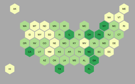
Below is the result of plotting the state populations (log scale):
One important property of visualizing data in maps is familiarity of the location (you can easily find specific states because you remember where they are) and also adjacency patterns can provide insights. For example, if we plot a measure as a choropleth map and see that the West coast is colored differently from the Midwest, then we gain an insight we wouldn’t have by looking at a column chart for example.
Because of this, ideally the homogeneous area maps should preserve adjacencies as much as possible. With that in mind, we can come up with a similarity score. Let X be the set of pairs of states that share a border in the actual US map. Now, let Y be the set of pairs of states that share a border in the hexagonal map (that is, two hexagons sharing a side). The similarity score is the size of their symmetric difference and we can normalize by the size of the original:
\[(\mid X - Y \mid + \mid Y - X \mid) / \mid X \mid\]The lower the score the better. In an ideal case, the borders sets would match perfectly for a score of 0.
The size of the symmetric difference between the two sets seems like a good measure for similarity, but I’m not sure about the normalization factor. I initially picked the size of the union of X and Y, but this wouldn’t let us model this problem as a linear programming model as we’ll see next. The problem with using the size of X is that the score could theoretically be larger than 1, but it’s trivial to place the hexagons in the grid in such a way that none of them are touching and thus Y is empty, so we can assume the score is between 0 and 1.
The score from the NPR maps is 0.67.
An Optimization Problem
Let’s generalize and formalize the problem above as follows: given a graph \(G = (V,E)\), and another graph \(H = (V_H, E_H)\) representing our grid, find the induced subgraph of \(H\), \(I = (V_I, E_I)\), such that there’s bijection \(f: V \rightarrow V_I\) and the size of the symmetric difference of \(f(E)\) and \(E_I\) is minimized (\(f(E)\) is an abuse of notation, but it means applying the bijection to each vertex in the set of edges \(E\)).
To make it clearer, let’s apply the definition above to the original problem. \(G\) represents the adjacency of states in the original map. \(V\) is the set of states and \(E\) is the set of pairs of states that share a border. \(H\) is the hexagonal grid. \(V_H\) is the set of all hexagons and \(E_H\) is the set of pairs of hexagons that are adjacent. We want to find a subset of the hexagons where we can place each of the states (hence the bijection from states to hexagons) and if two hexagons are in the grid, and we place two states there, we consider the states to be adjacent, hence the need for an induced graph, so the adjacency in the grid is preserved.
Is this general case an NP-hard problem? We can reduce the Graph Isomorphism problem to this one. It consists in deciding whether two graphs \(A\) and \(B\) are isomorphic. If we set \(G = A\) and \(H = B\), then \(A\) and \(B\) are isomorphic if and only if \(I = H\) and the symmetric difference of \(f(E)\) and \(E_I\) is 0. The problem is that it’s not known whether Graph Isomorphism belongs to NP-Complete.
What if \(G\) is planar (which is the case for maps)? I haven’t given much thought about it, but I decided to come up with an integer programming model nevertheless.
An Integer Linear Programming Model
Note: the model uses the original grid analogy instead of the more general problem so that the constraints are easier to understand.
Boolean algebra as linear constraints
Before we start, we need to recall how to model logical constraints (AND, OR and EQUAL) using linear constraints. Let a and b be binary variables. We want x to be the result of logical operators applied to a and b.
For AND, we can do (\(x = 1\) if and only if \(a = 1\) and \(b = 1\))
\(x \le a\) \(x \le b\) \(x \ge a + b - 1\)
For OR, we can do (\(x = 0\) if and only if \(a = 0\) and \(b = 0\))
\(x \ge a\) \(x \ge b\) \(x \le a + b\)
For EQUAL, we can do (\(x = 1\) if and only if \(a = b\))
\(x \le 1 - (a - b)\) \(x \le 1 - (b - a)\) \(x \ge a + b - 1\) \(x \ge -(a + b - 1)\)
We can introduce a notation and assume these constraints can be generated by a function. For example, if we say \(x = \mbox{EQ}(a, b)\), we’re talking about the four constraints we defined above for modeling EQUAL. This is discussed in [2].
Constants
Let \(G\) be the set of pairs \((x,y)\) representing the grid positions. Let \(P\) be the set of pieces \(p\) that have to be placed in the grid. Let \(N(x,y)\) be the set of pairs \((x',y')\) that are adjacent to \((x, y)\) in the grid.
Let \(A_{v1, v2}\) represent whether \(v1\) and \(v2\) are adjacent to each other in the dataset.
“Physical” constraints
Let \(b_{x,y,s}\) be a binary variable, and equals 1 if and only if state \(s\) is placed position \((x, y)\).
1) A piece has to be placed in exactly one spot in the grid:
\(\sum_{(x,y) \in G} b_{x,y,p} = 1\) for all \(p \in P\)
2) A spot can only be occupied by at most one state:
\(\sum_s b_{x,y,s} \le 1\) for all \((x,y) \in G\)
Adjacency constraints
Let \(a_{p1, p2, x, y}\) be a binary variable and equals 1 if and only if piece p1 is placed in \((x, y)\) and adjacent to \(p2\) in the grid.
3) \(a_{p1, p2, x, y}\) has to be 0 if \(p1\) is not in \((x,y)\) or \(p2\) is not adjacent to any of \((x,y)\) neighbors:
\[a_{p1, p2, x, y} = \mbox{AND}(\sum_{(x', y') \in N(x, y)} b_{x', y', p2}, b_{x,y,p})\]We have that \(a_{p1, p2, x, y}\) is 1 if and only if p1 is in \((x,y)\) and p2 is adjacent to any of \((x,y)\) neighbors.
Finally, we can model the adjacency between two pieces \(p1\) and \(p2\). Let \(a_{p1, p2}\) be a binary variable and equals 1 if and only if \(p1\) and \(p2\) are adjacent in the grid:
\[a_{p1, p2} = \sum_{(x,y) in G} a_{p1, p2, x, y}\]Symmetric difference constraints
Let \(y_{p1, p2}\) be a binary variable and equals to 1 if and only if \(a_{p1, p2} \ne A_{p1, p2}\).
4) \(y_{p1, p2} \ge a_{p1, p2} - A_{p1, p2}\) 5) \(y_{p1, p2} \ge A_{p1, p2} - a_{p1, p2}\)
Objective function
The sum of all \(y\)’s is the size of the symmetric difference:
\(\min \sum_{p1, p2 \in P} y_{p1, p2}\).
Practical concerns
This model can be quite big. For our US map example, we have \(\mid P \mid = 50\) and we need to estimate the size of the grid. A 50x50 grid is enough for any type of arrangement. The problem is that the number of variables \(a_{p1, p2, x, y}\) is \(\mid P \mid^2\mid G \mid = 50^4\) which is not practical.
We can also solve the problem for individual connected components in the original graph and it’s trivial construct the optimal solution from each optimal sub-solution. This doesn’t help much in our example, since only Hawaii and Alaska are disconnected, so we have |P| = 48. The grid could also be reduced. It’s very unlikely that an optimal solution would be a straight line. In the NPR map, the grid is 8x12. Sounds like doubling these dimensions would give the optimal solution enough room, so \(\mid G \mid = 8*12*4 = 384\).
We can also assume states are orderer and we only have variables \(a_{p1, p2, x, y}\) for \(p1 < p2\), so the number of \(a_{p1, p2, x, y}\) is about 450K. Still too large, unfortunately.
Another important optimization we can do in our case because we're working with a grid is to define the adjacency for x and y independently and combine them afterwards.
Refined adjacency constraints
Instead of working with \(b_{x,y,s}\) we use \(X_{x, s}\), and equals 1 if and only if state \(s\) is placed position \((x, y)\) for any y and \(Y_{y, s}\), which equals 1 iff state \(s\) is placed position \((x, y)\) for any x. The physical constraints are analogous to the previous model:
6) A piece has to be placed in exactly one spot in the grid:
\(\sum_{x \in G} X_{x,p} = 1\) for all \(p \in P\)
\(\sum_{y \in G} Y_{y,p} = 1\) for all \(p \in P\)
7) A spot can only be occupied by at most one state:
\(\sum_s X_{xs} \le 1\) for all \(x \in G\)
\(\sum_s Y_{y,s} \le 1\) for all \(y \in G\)
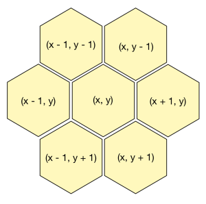
In a hexagonal grid, if we have the piece p1 in position \((x,y)\), it will be adjacent to another piece p2 if and only if p2 is in one of these six positions: 1: \((x-1, y)\), 2: \((x+1, y)\), 3: \((x-1, y-1)\), 4: \((x, y-1)\), 5: \((x-1, y+1)\) or 6: \((x, y+1)\). We can define two adjacency categories: Type I, which happens when \(p1.y - p2.y = 0\) and \(\mid p1.x - p2.x \mid = 1\) (cases 1 and 2); and Type II, which is when \(\mid p1.y - p2.y \mid = 1\) and \(p1.x - p2.x \le 0\) (cases 3, 4, 5 and 6).
Let’s define \(Y_{d=0, p1, p2, y} = 1\) iff \(p1.y - p2.y = 0\) for a given y. Similarly we define \(X_{\mid d \mid=1, p1, p2, x} = 1\) iff \(\mid p1.x - p2.x \mid = 1\), \(Y_{\mid d \mid=1, p1, p2, y} = 1\) iff \(\mid p1.y - p2.y \mid = 1\) and finally \(X_{d \ge 0, p1, p2, x} = 1\) iff \(p1.x - p2.x \ge 0\).
8) We can have the following constraints do model the variables we just defined:
\[Y_{d=0, p1, p2, y} = \mbox{EQ}(Y_{y, p_1}, Y_{y, p2})\] \[X_{\mid d \mid=1, p1, p2, x} = \mbox{EQ}(X_{x, p1}, X_{x-1, p2} + X_{x+1, p2})\] \[Y_{\mid d \mid=1, p1, p2, y} = \mbox{EQ}(Y_{y, p1}, Y_{y-1, p2} + Y_{y+1, p2})\] \[X_{d \ge 0, p1, p2, x} = \mbox{EQ}(X_{x, p1}, X_{x, p2} + X_{x+1, p2})\]9) Let \(Y_{d=0, p1, p2} = 1\) iff \(p1.x - p2.y = 0\) for any y. We can define analogous variables for the other cases:
\[Y_{d=0, p1, p2} = \sum_{y} Y_{d=0, p1, p2, y}\] \[X_{\mid d \mid=1, p1, p2} = \sum_{x} X_{d=0, p1, p2, x}\] \[Y_{\mid d \mid=1, p1, p2} = \sum_{y} Y_{d=0, p1, p2, y}\] \[X_{d \ge 0, p1, p2} = \sum_{x} Y_{d \ge 0, p1, p2, x}\]10) Let \(T'_{p1, p2} = 1\) iff p1 and p2 have the Type I adjacency and \(T''_{p1, p2} = 1\) iff p1 and p2 have Type II adjacency:
\[T'_{p1, p2} = \mbox{AND}(Y_{d=0, p1, p2}, X_{\mid d \mid=1, p1, p2})\] \[T''_{p1, p2} = \mbox{AND}(Y_{\mid d \mid=1, p1, p2}, X_{d \ge 0, p1, p2})\]11) Finally, we say that p1 and p2 are adjacency iff either Type I or Type II occurs:
\[a_{p1, p2} = \mbox{OR}(T'_{p1, p2}, T''_{p1, p2})\]The model for adjacency became much more complicated but we were able to reduce the number of adjacency variables are now roughly \(O(\mid P \mid^2 \sqrt{\mid G \mid})\). The number of non-zero entries in the right hand size of (which represents the size of the sparse matrix) is roughly 11M, dominated by the type (8) constraints. I’m still not confident this model will run, so I’ll punt on implementing it for now.
Conclusion
In this post we explored a different way to visualize the US states map. I was mainly exploring the idea of how good of an approximation this layout is and a natural question was how to model this as an optimization problem. Turns out that if we model it using graphs, the problem definition is pretty simple and happens to be a more general version of the Graph Isomorphism problem.
I struggled with coming up with an integer programming model and couldn’t find one with a manageable size, but it was a fun exercise!
World Map?
One cannot help wondering if we can display the countries in a hexagonal map. I’m planning to explore this idea in a future post. The main challenge is that the US states areas are more uniform than the countries. For example, the largest state (Alaska) is 430 times larger than the smallest (Rhode Island). While the largest country (Russia) is almost 40,000,000 bigger than the smallest (Vatican City).
Also, the layout of the US map was devised by someone from NPR and they did a manual process. I’m wondering if we can come up with a simple heuristic to place the hexagons and then perform manual adjustments.
References
- [1] NPR Visuals Team - Let’s Tesselate: Hexagons For Tile Grid Maps
- [2] Computer Science: Express boolean logic operations in zero-one integer linear programming (ILP)
- [3] SOM - Creating hexagonal heatmaps with D3.js
- [4] Github - d3/d3-hexbin
Data sources
