kuniga.me > NP-Incompleteness > Notes on Javascript Memory Profiling in Google Chrome
Notes on Javascript Memory Profiling in Google Chrome
07 Jun 2015
In this post we’ll explore the topic of Javascript memory management, in particular in Google Chrome. This post is based on a talk by Loreena Lee and John McCutchan at Google I/O 2013.

We’ll start by covering some aspects of Google Chrome architecture and then describe some of the main tools it offers for analyzing and debugging memory.
For the experiments, we used Chrome Canary, version 45.0 in a Mac.
Graph representation
The browser maintains a graph representation of its objects. Each node represents an object and directed arcs represent references. There are three types of nodes:
- Root node (e.g. the window object in the browser)
- Object node
- Scalar nodes (primitive types)
We define shallow size as the amount of memory used by the object itself (not counting the size of references).
The retaining path of a node is a directed path from the root to that node. This is used to determine whether a node is still being used, because otherwise it can be garbage collected. The retained size of a node is the amount of memory that would be freed if it was removed (includes the memory from nodes that would be deleted with this node).
A node u is a dominator of a node v, is it belongs to every single path from the root to v.
V8 memory management
V8 is the JavaScript engine that powers Google Chrome. In this section, we’ll describe some of its characteristics.
Data types representation
JavaScript has a few primitive data types. The spec describes them but does not dictates how they should be represented in memory.
This may differ from JavaScript engine to engine. Let’s briefly describe how V8 handles that, according to Jay Conrod [2]:
-
Numbers: can be represented as Small Integers (SMIs) if they represent integers, using 32 bits. If the number is used as a double type or needs to be boxed (for example, use properties like
toString()), they are stored as heap objects. -
Strings can be stored in the VM heap or externally, in the renderer’s memory, and a wrapper object is created. This is useful for representing script sources and other content that is received from the Web.
-
Objects are key-value data structures, where the keys are strings. In practice they can be represented as hash tables (dictionary mode) or more efficient structures when objects share properties with other objects or when they are used as arrays. A more in depth study of these representations can be seen in [2].
-
DOM elements and images are not a basic type of V8. They are an abstraction provided by Google Chrome and external to V8.
Garbage collection
Objects get allocated in the memory pool until it gets full. At this point, the garbage collector is triggered. It’s a blocking process, so this process is also called the GC pause, which can last for a few milliseconds.
Any object that is not reached from the root can be garbage collected. V8 classify the objects in two categories in regards of garbage collection: young and old generations.
All allocated objects start as young generation. As garbage collections occur, objects that were not removed are moved to the old generation. Young generation objects are garbage collected much more often than old objects.
It’s an optimization that makes sense. Statistically, if an object “survived” to many garbage collections, they are less likely to be collected, so we can make these checks less often.
Now that we have a basic understanding of how Chrome deals with memory, we can learn about some of the UI tools it has for dealing with memory.
The task Manager
This tool displays a list of tabs and extensions currently running in your browser. It contains useful information like the amount of Javascript memory each one is using.
https://developer.chrome.com/devtools/docs/javascript-memory-profiling#chrome-task-manager
The timeline tool
The timeline tool allow us to visualize the amount of memory used over time. The dev tools docs contain an example where we can try out the tool:
https://developer.chrome.com/devtools/docs/demos/memory/example1
We’ll obtain a result similar to this:
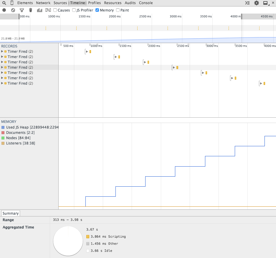
In the “Memory” tab, we can see counts like number of documents, event listeners, DOM nodes and also the amount of memory in the JavaScript heap.
The reason we need a separate count is that DOM nodes use native memory and do not directly affect the JavaScript memory graph [3].
The profile tool - Heap Snapshot
The heap snapshot dumps the current memory into the dev tools for analysis. It offers different views: Summary, Comparison, Containment and Statistics.
The statistics is just a pie chart showing a break down of objects by their types. Not much to see here. Let’s focus on the other three.
1. Summary view
This is the default view. It’s a table representing a tree structure, like the one below.

We can observe the table above contains the following columns:
- Constructor - the name of the function used to instantiate an object.
- Distance - represents the distance of the corresponding nodes to the root (try sorting by distance. You’ll see the Window objects with distance 1).
- Objects Count - the number of objects created with that particular constructor
- Shallow Size - the amount of memory in bytes an object is using
- Retained Size - accounts for all memory an object refers to
If we follow the example in the docs:
https://developer.chrome.com/devtools/docs/heap-profiling-summary
And take a snapshot, we can locate the Item constructor. We see ~20k objects created and their shallow size (each has 32 bytes).

Detached nodes. Nodes that are not part of the main DOM tree (rooted in the <html /> element) are considered detached. In the example below, we could have a DOM element with ID ‘someID’ and remove it from the main DOM tree.
var refA = document.getElementById('someID');
document.body.removeChild(refA);
At this point it’s considered detached, but it can’t be garbage collected because the variable refA still refers to it (and could potentially reinsert the node back later). If we set refA to null and no other variable refers to it, it can be garbage collected.
Moreover, the someID node might have child nodes that would also not be garbage collected, even though no JavaScript variable refers to it directly (it does indirectly through the refA).
In the profile table, detached nodes that are directly referenced by some JavaScript variable have a yellow background and those indirectly references have a red background.
In the table below, we can see some yellow and red colored nodes:

Object IDs. When we do a profiling, the Dev tools will attach an ID to each Javascript object and those are displayed in the table to the right of the constructor name, in the form @12345 where 12345 is the ID generated for the object. These IDs are only generated if a profile is made and the same object will have the same ID across multiple profilings.
2. Comparison view.
This view allows comparing two snapshots. The docs also provide an example to try out this tool:
https://developer.chrome.com/devtools/docs/heap-profiling-comparison
If we follow the instructions, we’ll get something like:

We can see the Delta column, showing the difference in number of objects compared to the previous snapshot, which could help with a memory leak investigation. We also have the amount of memory added (Alloc. Size), freed (Freed Size) and the net difference (Size Delta).
3. Containment view.
The containment view organizes the objects by hierarchy. At the top level we can see several Window objects, one of those corresponding to the page we’re looking. For example, if we take a snapshot of the following page:
https://developer.chrome.com/devtools/docs/heap-profiling-containment
And switch the view to Containment, we’ll see something like:

The profile tool - Heap allocation
The heap allocation tool (also referred as Object Allocation Tracker in the docs) takes snapshots at regular intervals until we stop recording.
It plots a timeline of bars corresponding to memory allocated during that snapshot. The blue portion displays the amount of memory created during that snapshot that is still alive. The gray portion depicts the memory that has been released since then.
We can do a simple experiment to see this behavior in practice. We create two buttons: one that allocates some memory and append to a given DOM node and another that removes one child of the node. The code for this setup can be found on github/kunigami.
If we keep playing with the buttons while recording, we can see blue bars being created when we click “Append” and graying out when we click “Remove”.

Conclusion
Google Chrome offers many tools for memory diagnosing and it can be overwhelming to decide which one to use. The timeline view is a good high-level tool to detect memory patterns (especially memory leaks).
After that is spotted, the profiling tools can give more details on what is being allocated. This tool displays a lot of information, which can also be hard to read.
The comparison view is useful in these cases because it only show differences.
The documentation is a bit sparse, but contains good examples to try out the tools. These examples have some instructions on how to use the tools, but usually lack screenshots of the results.
