kuniga.me > NP-Incompleteness > Supervised Machine Learning
Supervised Machine Learning
04 Jun 2014

Andrew Ng is a Computer Science professor at Stanford. He is also one of the co-founders of the Coursera platform. Andrew recently joined the Chinese company Baidu as a chief scientist.
His main research focus is on Machine Learning, Artificial Intelligence and Deep Learning. He teaches the Machine Learning class in Coursera, which lasts 10 weeks and is comprised of videos, multiple choice assignments and programming assignments (with Octave).
Professor Andrew is a very good lecturer and makes the content more accessible by relying more on intuition rather than rigor, but always mentioning that a given result is backed by mathematical proofs. The material is very practical and he often discusses about real world techniques and applications.
Throughout the classes I got curious about the math behind many of the results he presented, so this post is an attempt to help me with that, as well as providing a overview of the content of the course.
Supervised Learning

Suppose we have a set of data points and each of these points encodes information about a set of features, and for each of these vectors we are also given a value or label, which represents the desired output. We call this set a training set.
We want to find a black box that encodes some structure from this data and is able to predict the output of a new vector with certain accuracy.
It’s called supervised because we require human assistance in collecting and labeling the training set. We’ll now discuss some methods for performing supervised learning, specifically: linear regression, logistic regression, neural networks and support vector machines.
Linear regression
We are given a set \(X\) of \(m\) data points, where \(x_i \in R^n\) and a set of corresponding values \(Y\), where \(y_i \in R\).
Linear regression consists in finding a hyperplane in \(R^n\), which we can represent by \(y = \Theta^{T} x\) (here the constant is represented by \(\Theta_0\) and we assume \(x_0 = 1\)), such that the sum of the square distances of \(y_i\) and the value of \(x_i\) in that hyperplane, that is, \(\Theta^{T} x_i\), for each \(i=1, \cdots, m\), is minimized.
More formally, we can define a function:
\[f_{X,Y}(\Theta) = \sum_{i=1}^{m} (y_i - \Theta^{T}x_i)^2\]We want to fit a hyperplane that minimizes \(f\). We can do so by finding the optimal parameters \(\Theta^{*}\):
\(\Theta^{*} = \min_{\Theta} f_{X, Y}(\Theta)\).
This linear regression with the least square cost function is also known as linear least squares.
We can solve this problem numerically, because it’s possible to show that \(f(\Theta)\) is convex. One common method is gradient descent (we used this method before for solving Lagrangian relaxation).
We can also find the optimal \(\Theta^{*}\) analytically, using what is known as the normal equation:
\[(X^T X) \Theta^{*} = X^T y\]This equation comes from the fact that a convex function has its minimum/maximum value when its derivative in terms of its input is 0. In our case, \(\dfrac{\partial f_{X, Y}}{\partial \Theta}(\Theta^{*}) = 0\).
The assumption is that our data lies approximately in a hyperplane, but in reality it might be closer to a quadratic curve. We can then create a new feature that is a power of one of the original features, so we can represent this curve as a plane in a higher dimension.
This method also returns a real number corresponding to the estimated value of \(y\), but many real world problems are classification problems, most commonly binary (yes/no). For this case linear regression doesn’t work very well. We’ll now discuss another method called logistic regression.
Logistic regression
In logistic regression we have \(y_i \in \{0, 1\}\) and the idea is that after trained, our model returns a probability that a new input belongs to the class \(y=1\).
Here we still train our model to obtain \(\Theta\) and project new input in the corresponding hyperplane to obtain a numerical value. But this time, we convert this to the range [0-1], by applying the sigmoid function, so it becomes
\[h_{\Theta}(x^{(i)}) = \dfrac{1}{1 - e^{(\Theta^T x^{(i)})}}\]This represents the probability that given \(x^{(i)}\) parametrized by \(\Theta\), the output will be 1, that is, \(p(y^{(i)}=1\mid x^{(i)}; \Theta)\). The probability of y being 0 is the complementary, that is
\[p(y^{(i)}=0\mid x^{(i)}; \Theta) = 1 - p(y^{(i)}=1\mid x^{(i)}; \Theta)\]The likelihood of the parameter \(\Theta\) to fit the data can be given by
(1) \(\ell(\Theta) = \prod_{i=1}^{m} (h_{\Theta}(x^{(i)}))^{y^{(i)}} (1 - h_{\Theta}(x^{(i)}))^{({1 - y^{(i)}})}\)
We want to find the maximum likelihood estimation (MLE), that is, the parameter \(\Theta\) that minimizes (1). We can apply the log function to the \(\ell(\Theta)\), because the optimal \(\Theta\) is the same in both. This get us
(2) \(- \left[\sum_{i=1}^{m} y^{(i)} \log (h_{\Theta}(x^{(i)})) + (1 - y^{(i)})\log(1 - h_{\Theta}(x^{(i)}))\right]\)
This function doesn’t allow a closed form, so we need a numerical algorithm, such as gradient descent. This function is not necessarily convex either, so we might get stuck in local optima.
After estimating the parameter \(\Theta^{*}\), we can classify a input point \(x\) by:
\[y = \left\{ \begin{array}{ll} 1 & \mbox{if } h_{\Theta^{*}}(x)) \ge 0.5 \\ 0 & \mbox{otherwise} \end{array} \right.\]Neural Networks
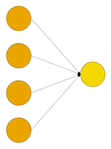
Neural networks can be seen as a generalization of the simple form of logistic regression seen above. In there, we have one output (\(y\)) that is a combination of several inputs (\(x_j\)). We can use a diagram to visualize it. More specifically, we could have a directed graph like the following:

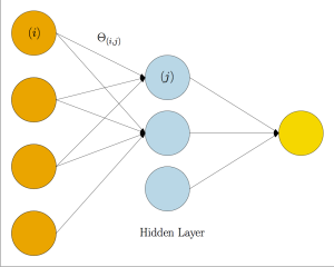
Here we have nodes representing the input data and the output and each edge as a corresponding parameter \(\Theta\). We can partition this graph in layers. In this case, the input and the output layer. In order to generalize that, we could add intermediate layers, which can be called hidden-layers:

In the general case, we have \(L\) layers. Between layers \(\ell\) an \(\ell+1\), we have a complete bipartite graph. Each edge \((i,j)\) connecting node \(i\) at level \(\ell\) to node \(j\) at level \(\ell+1\) is associated to a \(\Theta_{ij}^{(\ell)}\). The idea at each node it the same: perform the linear combination of the nodes incident to it and then apply the sigmoid function. Note that at each layer, we have one node that is not connected to any of the previous layers. This one acts as the constant factor for the nodes in the following layer. The last node will represent the final value of the function based on the input \(X\).
There’s a neat algorithm to solve this, called back-propagation algorithm.
Forward-propagation is the method of calculating the cost function for each of the nodes. The idea is the following. For each level \(\ell\) we’ll use variables \(a\) and \(z\).
Initialize \(a\):
\[a^{(0)} = x\]For the following layers \(\ell=1, \cdots, L\) we do:
\[\begin{array}{ll} z^{(\ell)} & = (\Theta^{(\ell-1)})^{T} a^{(\ell-1)}\\ a^{(\ell)} & = g(z^{(\ell)}) \end{array}\]for the simple case of binary classification, the last layer will contain a single node and after running the above procedure, it will contain the cost function for an input \(x\):
\[h_{\Theta}(x) = a^{(L)}\]Then, we can define the cost function \(J\) to be the average of (2) for the training set.
\(J(\Theta) = - \dfrac{1}{m} \left[\sum_{i=1}^{m} y^{(i)} \log (h_{\Theta}(x^{(i)})) + \right.\) \(\left. (1 - y^{(i)})\log(1 - h_{\Theta}(x^{(i)}))\right]\)
Back-propagation is the algorithm to find the derivatives of the cost function with respect to \(\Theta\). In this procedure, we use the helper variables \(\delta\), which we initialize as:
\[\delta^{(L)} = a^{(L)} - y^{(i)}\]We iterate over the layers backwards \(\ell = L-1, \cdots, 1\):
\[\delta^{(\ell)} = (\Theta^{(\ell)})^{T} \delta^{(\ell+1)} .* g'(z^{(i)})\]\(\delta\) is defined in such a way that
\[\dfrac{\partial J(\Theta)}{\partial \Theta_{j,k}^{(\ell)}} = \dfrac{1}{m} \sum_{i=1}^{m} a_{k}^{(\ell)} \delta_{j}^{(\ell+1)}\]For an sketch of the derivation of these equations, see the Appendix.
Support Vector Machine
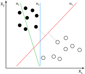
Support Vector Machine is a method for binary classification and it does so by defining a boundary that separates points from different classes. For this model, our labels are either \(y \in \{-1, 1\}\) (as opposed to \(y \in \{0, 1\})\).
In the simple case, where we want to perform a linear separation, it consists in finding a hyperplane that partitions the space in regions, one containing points with y=-1 and the other y=1; also, it tries to maximize the minimum distance from any point to this hyperplane.

Instead of working with the parameters \(\Theta\), we’ll have \(w\) and \(b\), so we can represent our hyperplane as \(w^Tx^{(i)} + b\). The classification function is give by:
\[h_{w,b}(x) = g(w^Tx + b)\]Where \(g\) is the sign function, that is, \(g(z) = 1\) if \(z \ge 0\) and \(g(z) = -1\) otherwise.
Margin
For each training example \(x^{(i)}\), we can define a margin as:
\[\gamma^{(i)} = y^{(i)} (w^Tx^{(i)} + b)\]Intuitively, a function margin represents the confidence that point \(x^{(i)}\) belongs to the class \(y^{(i)}\). Given \(m\) input points, we define the margin of the training set as
(3) \(\gamma = \min_{ i = 1, \cdots, m} \gamma^{(i)}\)
We then want to maximize the margin, so we can write the following optimization problem:
\[\max \gamma\]s.t. \(y^{(i)} (w^Tx^{(i)} + b) \ge \gamma\)
The constraint is to enforce (3). The problem with this model is that we can arbitrarily scale \(w\) and \(b\) without changing \(h_{w,b}(x)\), so the optimal solution is unbounded.
The alternative is to normalize the by dividing by \(\mid\mid w \mid\mid\), so it becomes indifferent to scaling.
Primal form
It’s possible to show that in order to maximize the margin, we can minimize the following linear programming with quadratic objective function:
\[\min \frac{1}{2} \mid\mid w \mid\mid^2\]s.t. \(y^{(i)}(w^Tx^{(i)} + b) \ge 1\), for \(i = 1, \cdots, m\)
Dual form
For non-linear programming, it’s possible to make use of Lagrangian multipliers to obtain the dual model. In particular, the following model obtained using this idea, together with the primal form, satisfy the Karush–Kuhn–Tucker (KKT) conditions, so the value of the optimal solution for both cases is the same.
\[\max_{\alpha} W(\alpha) = \sum_{i=1}^{m} \alpha_i - \frac{1}{2} \sum_{i,j=1}^{m} y^{(i)}y^{(j)} \alpha_i \alpha_j \langle x^{(i)}, x^{(j)} \rangle\]s.t. \(\begin{array}{llr} \alpha_i & \ge 0 & i=1,\cdots,m \\ \sum_{i=1}^{m} \alpha_i y^{(i)} & = 0 \end{array}\)
It’s possible to show that the non-zeros entries of \(\alpha_i\) correspond to the input points that will define the margin. We call these points support vectors.
Moreover, \(w\) can be obtained by the following equation:
\[w = \sum_{i=1}^{m} \alpha_i y^{(i)} x^{(i)}\]Non-linear SVM: Kernels
Kernel is a way to generate features from the training set. For example, we can generate \(m\) features from the \(m\) points in the training set by having feature \(f_i\) to be the similarity of a point to it. One common similarity function is the Gaussian distance. Given points \(x^{(i)}\) and \(x^{(j)}\), we can compute it by:
\[K_{\mbox{gaussian}}(x^{(i)}, x^{(j)}) = \exp \left(-\dfrac{\mid\mid x^{(i)} - x^{(j)}\mid\mid^2}{2\sigma^2}\right)\]Conclusion
I’ve completed an Artificial Intelligence class in college and previously did the PGM (Probabilistic Graphical Models). One of the main reasons I enrolled for this course was the topic of Support Vector Machines.
Unfortunately, SVM was discussed in a high level and apart from kernels, it was pretty confusing and mixed up with logistic regression. SVM happened to be a very complicated topic and I ended up learning a lot about it with this post, but I still don’t fully understand all the details.
References
- [1] Wikipedia: Back-propagation
- [2] Prof. Cosma Shalizi’s notes - Logistic Regression
- [4] Prof. Andrew Ng’s notes - Support Vector Machine
- [5] Wikipedia: Support Vector Machine
- [6] An Idiot’s guide to Support Vector Machines
Appendix: Derivation of the backpropagation relations
In this appendix we’ll calculate the partial derivative of \(J(\Theta)\) in relation to a \(\Theta_{ij}^{(\ell)}\) component to get some insight into the back-propagation algorithm. For simplicity, we’ll assume a single input \(x^{(i)}\), so we can get rid of the summation.
By the chain rule we have:
\[\dfrac{\partial J(\Theta)}{\partial \Theta_{j, k}^{(\ell)}} = \dfrac{\partial J(\Theta)}{\partial a^{(\ell)}} \cdot \dfrac{\partial a^{(\ell)}}{\partial z^{(\ell)}} \cdot \dfrac{\partial z^{(\ell)}}{\partial \Theta_{j,k}^{(\ell)}}\]Let’s analyze each of the terms:
For the term \(\dfrac{\partial z^{(l)}}{\partial \Theta_{j,k}^{(\ell)}}\), we have that \(z^{(\ell)} = \Theta^{(\ell)} a^{(\ell-1)}\) or breaking down by elements:
\[z^{(\ell)}_{k'} = \sum_{j=1}^{n^{(\ell-1)}} \Theta^{(\ell)}_{j,k'} a^{(\ell-1)}_j\]For \(k=k'\), it’s easy to see that \(\dfrac{\partial z^{(\ell)}_k}{\partial \Theta_{j,k}^{(\ell)}} = a^{(\ell-1)}_j\). For \(k \ne k'\),
\[\dfrac{\partial z^{(\ell)}_{k'}}{\partial \Theta_{j,k}^{(\ell)}} = 0\]For the term \(\dfrac{\partial a^{(\ell)}}{\partial z^{(\ell)}}\), we have that \(a^{(\ell)} = g(z^{(\ell)})\), thus, \(\dfrac{\partial a^{(\ell)}}{\partial z^{(\ell)}} = g'(z^{(\ell)})\)
Finally, for the term \(\dfrac{\partial J(\Theta)}{\partial a^{(\ell)}}\), we will assume that \(J(\Theta) \approx \dfrac{1}{2} (a^{(\ell)} - y)^2\)
If \(\ell = L\), then \(a^{(\ell)} = h_\Theta(x)\), so it’s the derivative is straightforward:
\[\dfrac{\partial J(\Theta)}{\partial a^{(L)}} = (h_\Theta(x) - y)\]For the intermediate layers, we can find the derivative by writing it in terms of subsequent layers and then applying the chain rule. Inductively, suppose we know \(\dfrac{\partial J(\Theta)}{\partial a^{(\ell)}}\) (base is \(\ell = L\)) and we want to find \(\dfrac{\partial J(\Theta)}{\partial a^{(\ell - 1)}}\). We can write:
(4) \(\dfrac{\partial J(\Theta)}{\partial a^{(\ell - 1)}} = \dfrac{\partial J(\Theta)}{\partial a^{(\ell)}} \cdot \dfrac{\partial a^{(\ell)}}{\partial a^{(\ell - 1)}}\)
Given that \(a^{(\ell)} = g(z^{(\ell)}) = g((\Theta^{(\ell-1)})^T a^{(\ell - 1)})\), we have:
\[\dfrac{\partial a^{(\ell)}}{\partial a^{(\ell - 1)}} = \dfrac{\partial a^{(\ell)}}{\partial z^{(\ell)}} \cdot \dfrac{\partial z^{(\ell)}}{\partial a^{(\ell - 1)}} = (\Theta^{(\ell - 1)})^T \dfrac{\partial a^{(\ell)}}{\partial z^{(\ell)}}\]Replacing back in (4):
\[\dfrac{\partial J(\Theta)}{\partial a^{(\ell - 1)}} = \dfrac{\partial J(\Theta)}{\partial a^{(\ell)}} \cdot (\Theta^{(\ell -1)})^T \dfrac{\partial a^{(\ell)}}{\partial z^{(\ell)}} = (\Theta^{(\ell -1)})^T \dfrac{\partial J(\Theta)}{\partial z^{(\ell)}}\]If we name \(\delta^{(\ell)} = \dfrac{\partial J(\Theta)}{\partial z^{(\ell)}}\), we now have
(5) $$ \dfrac{\partial J(\Theta)}{\partial a^{(\ell - 1)}} =
(\Theta^{(\ell -1)})^T \delta^{(\ell)} $$
“Undoing” one of the chain steps, we have
\[\dfrac{\partial J(\Theta)}{\partial z^{(\ell-1)}} = \dfrac{\partial J(\Theta)}{\partial a^{(\ell-1)}} \cdot \dfrac{\partial a^{(\ell-1)}}{\partial z^{(\ell-1)}}\]Replacing (5) here,
$$
(\Theta^{(\ell -1)})^T \delta^{(\ell)} \dfrac{\partial a^{(\ell-1)}}{\partial z^{(\ell-1)}} $$
With that, we can get the following recurrence:
\[\delta^{(\ell-1)} = (\Theta^{(\ell-1)})^T \delta^{(\ell)} g'(z^{(\ell - 1)})\]Finally, replacing the terms in the original equation give us
\[\dfrac{\partial J(\Theta)}{\partial \Theta_{j, k}^{(\ell)}} = \dfrac{\partial J(\Theta)}{\partial a^{(\ell)}} \cdot \dfrac{\partial a^{(\ell)}}{\partial z^{(\ell)}} \cdot \dfrac{\partial z^{(\ell)}}{\partial \Theta_{j,k}^{(\ell)}} = a_j^{(\ell)} \delta_k^{(\ell+1)}\]