kuniga.me > NP-Incompleteness > The Algorithm X and the Dancing Links
The Algorithm X and the Dancing Links
28 Apr 2013
Introduction
In a Donald Knuth’s paper called Dancing Links [1], he shows an algorithm that can be used to solve puzzles like Sudoku via backtracking in a efficient way.
The backtracking algorithm is named simply the Algorithm X for a lack of a better name [1] and because it’s very simple and not the focus of the paper.
The main concept is actually a data structure used to implement the algorithm X. It’s a sparse matrix where Knuth uses some clever tricks to make removing/restoring columns and rows efficient and in-place operations. He refers to these operations as dancing links, in allusion to how the pointers from the cells change during these operations.
In this post we’ll describe in more details the problem we are trying to solve and then present the idea of the algorithm X. We’ll follow with the description of the data structure and how the mains steps of the algorithm can be implemented using dancing links.
Finally, we’ll present a simple example implementation on Python.
Set Cover
The Sudoku puzzle can be modeled as a more general problem, the set cover problem.
Given a set of items U and a set S of sets each of which covering some subset of U, the set cover problem consists in finding a subset of S such that each element is covered by exactly one set. This problem is known to be NP-Complete.
The set cover can be viewed as a binary matrix where the columns represent the elements to be covered and the rows represent the sets. An entry 1 in the cell i,j, means that the set i covers element j.
The objective is then finding a subset of the rows such that for each column, there is exactly one entry of 1.
In fact, this is the constraint matrix of a common integer linear programming formulation for this problem.
The Algorithm X
Knuth’s algorithm performs a full search of all possible solutions recursively, in such a way that at each node of the search tree we have a submatrix representing a sub-problem.
At a given node, we try adding a given set for our solution. We then discard all elements covered by this set and also discard all other sets that cover at least one of these elements, because by definition one element can’t be covered by more than one set, so we are sure these other sets won’t be in the solution. We then repeat the operation on the remaining subproblem.
If, at any point, there’s an element that can’t be covered by any set, we backtrack, trying to pick a different set. On the other hand, if we have no element left, our current solution is feasible.
More formally, at a given node of the backtrack tree, we have a matrix binary \(M\). We first pick some column \(j\). For each row \(i\) such that \(M_{ij} = 1\), we try adding i to our current solution and recurse over a submatrix \(M'\), constructed by removing from \(M\) all columns j' such that \(M_{ij'} = 1\), and all rows \(i'\) such that \(M_{i'k} = M_{ik} = 1\) for some column \(k\).
Dancing Links
A naive implementation of the above algorithm would scan the whole matrix to generate the submatrix and it would store a new matrix in each node of the search tree.
Knuth’s insight was to represent the binary matrix as a doubly linked sparse matrix. As we’ll see later, this structure allows us to undo the operations we do for the recursion, so we can always work with a single instance of such sparse matrix.
The basic idea of a sparse matrix is creating a node for each non-zero entry and linking it its adjacent cells on the same column and to adjacent cells on the same line.
In our case, our nodes (depicted in green in Fig. 1) are doubly linked and form a circular chain. We also have one header node (blue) for each column that is linked to the first and last nodes of that column and a single header (yellow) that connects the header of the first column and the last one.
Here’s an example for the matrix \(\begin{pmatrix}0 & 1\\1 & 1\end{pmatrix}\):
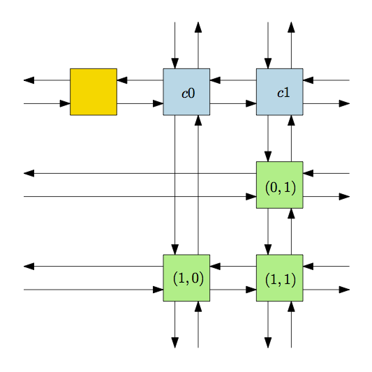
Note that the pointers that are coming/going to the border of the page are circular.
For each node we also have a pointer to the corresponding header of its column.
Removing a node. A known way to remove or de-attach a node from a doubly linked circular list is to make its neighbors to point to each other:
node.prev.next = node.next
node.next.prev = node.prev
Restoring a node. Knuth tells us that it’s also possible to restore or re-attach a node to its original position assuming we didn’t touch it since the removal:
node.prev = node
node.next = node
Removing a column. For our algorithm, removing a column is just a matter of de-attaching its corresponding header from the other headers (not from the nodes in the column), so we call this a horizontal de-attachment.
Removing a row. To remove a row, we want to de-attach each node in that row from it’s vertical neighbors, but we are not touching the links between nodes of the same row, so we call this a vertical de-attachment.
A Python implementation
We’ll present a simple implementation of these ideas in Python. The complete code can be found on Github.
Data Structures
Our basic structures are nodes representing cells and heads representing columns (and also a special head sentinel). We need all the four links (left, up, right, down), but we don’t need to declare them explicitly because python allow us to set them dynamically. We will have an additional field pointing to the corresponding header. The main difference is that we only attach/de-attach nodes vertically and heads horizontally, so we have different methods for them:
class Node:
    def __init__(self, row, col):
        self.row, self.col = row, col

    def deattach(self):
        self.up.down = self.down
        self.down.up = self.up

    def attach(self):
        self.down.up = self.up.down = self

class Head:
    def __init__(self, col):
        self.col = col

    def deattach(self):
        self.left.right = self.right
        self.right.left = self.left

    def attach(self):
        self.right.left = self.left.right = self
Now we need to build our sparse matrix out of a regular python matrix. We basically create one node for each entry 1 in the matrix, one head for each column and one global head. We then link them with helper functions:
class SparseMatrix:

    def createLeftRightLinks(self, srows):
        for srow in srows:
            n = len(srow)
            for j in range(n):
                srow[j].right = srow[(j + 1) % n]
                srow[j].left = srow[(j - 1 + n) % n]

    def createUpDownLinks(self, scols):
        for scol in scols:
            n = len(scol)
            for i in range(n):
                scol[i].down = scol[(i + 1) % n]
                scol[i].up = scol[(i - 1 + n) % n]
                scol[i].head = scol[0]

    def __init__(self, mat):

        nrows = len(mat)
        ncols = len(mat[0])

        srow = [[ ] for _ in range(nrows)]
        heads = [Head(j) for j in range(ncols)]
        scol = [[head] for head in heads]

        # Head of the column heads
        self.head = Head(-1)
        heads = [self.head] + heads

        self.createLeftRightLinks([heads])

        for i in range(nrows):
            for j in range(ncols):
                if mat[i][j] == 1:
                    node = Node(i, j)
                    scol[j].append(node)
                    srow[i].append(node)

        self.createLeftRightLinks(srow)
        self.createUpDownLinks(scol)
Iterators
We were repeating the following code in several places:
it = node.left
while it != node:
  # Do some stuff
  it = it.left
With left eventually replaced by right, up or down. So we abstract that using an iterator:
class NodeIterator:

    def __init__(self, node):
        self.curr = self.start = node

    def __iter__(self):
        return self

    def next(self):
        _next = self.move(self.curr)
        if _next == self.start:
            raise StopIteration
        else:
            self.curr = _next
            return _next

    def move(self):
        raise NotImplementedError
This basically goes through a linked list using a specific move operation. So we can implement specific iterators for each of the directions:
class LeftIterator (NodeIterator):
    def move(self, node):
        return node.left

class RightIterator (NodeIterator):
    def move(self, node):
        return node.right

class DownIterator (NodeIterator):
    def move(self, node):
        return node.down

class UpIterator (NodeIterator):
    def move(self, node):
        return node.up
Then, our previous while block becomes
for it in LeftIterator(node):
  # Do some stuff
Algorithm
With our data structures and syntax sugar iterators set, we’re ready to implement our backtracking algorithm.
The basic operation is the covering and uncovering of a column. The covering consists in removing that column and also all the rows from its row list (remember that a column can only be covered by exactly one row, so we can remove the other rows from the candidate list).
class DancingLinks:

    def cover(self, col):
        col.deattach()
        for row in DownIterator(col):
            for cell in RightIterator(row):
                cell.deattach()

    def uncover(self, col):
        for row in UpIterator(col):
            for cell in LeftIterator(row):
                cell.attach()
        col.attach()

   ...
When covering a row of a column col, we start from the column to the right of col and finish at the column on its left, thus, we don’t actually de-attach the cell from col from its vertical neighbors. This is not needed because we are already “removed” the column from the matrix and this allow us to make a more elegant implementation.
It’s important the uncover to do the operations in the reverse other of the cover so we won’t mess with the pointers in the matrix.
The main body of the algorithm is given below, which is essentially the definition of the Algorithm X, that returns true whenever it has found a solution.
    def backtrack(self):
        # Let's cover the first uncovered item
        col = self.smat.head.right
        # No column left
        if col == self.smat.head:
            return True
        # No set to cover this element
        if col.down == col:
            return False

        self.cover(col)

        for row in DownIterator(col):

            for cell in RightIterator(row):
                self.cover(cell.head)

            if self.backtrack():
                self.solution.append(row)
                return True

            for cell in LeftIterator(row):
                self.uncover(cell.head)

        self.uncover(col)

        return False
Knuth notes that in order to reduce the expected size of the search tree we should minimize the branching factor at earlier nodes by selecting the columns with more 1 entries, which will throw the most number of candidate rows away. But for the sake of simplicity we are choosing the first one.
Conclusion
In this post we revisited concepts like the set cover problem and the sparse matrix data structure. We saw that with a clever trick we can remove and insert rows and columns efficiently and in-place.
Complexity
Suppose that in a given node we have a \(n \times m\) matrix. In the naive approach, for each candidate row we need to go through all of the rows and columns to generate a new matrix, leading to a \(O(n^2m)\) complexity for each node.
In the worst case, using a sparse matrix will lead to the same complexity, but hard set cover instances are generally sparse, so in practice we may have a performance boost. Also, since we do everything in-place, our memory footprint is considerably smaller.
Related Posts
Mentioned by Buddy Memory Allocation.
