kuniga.me > NP-Incompleteness > Probabilistic Graphical Model Lecture Notes - Week 9
Probabilistic Graphical Model Lecture Notes - Week 9
21 May 2012
This post contains my notes for week 9, the last of the Probabilistic Graphical Models online course.
Learning from incomplete data
Overview
In practice, the samples we work with are often incomplete, and may be due to failures in data acquisition or even the presence of latent (hidden) variables in the model.
As a reminder, we used latent variables in the model to simplify it. Consider the example below:
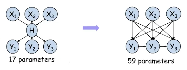
In the example we can see that the introduction of the variable $H$ reduces the number of edges in the model and consequently the number of parameters.
Dealing with incomplete data
We can consider two cases of missing information. If it occurs independently of the observed value, then we just ignore samples with incomplete data. On the other hand, if there is a dependency between the missing information and the observed value, then we cannot simply ignore incomplete samples. In this case we need to consider the mechanism that models the loss of this data.
Missing At Random (MAR) is when the probability of missing data is independent of its value. A simple example is when we sample coin flips. If in random occasions we fail to record the result of a toss, then we have a MAR.
On the other hand, if for some reason we only fail to record tosses that resulted in heads, then the probability of missing data is influenced by the sample value and in this case we do not have a MAR.
With incomplete data, the likelihood function has multiple local optima. An intuition is that by replacing a missing sample value with any value, the likelihood value remains the same, although the point in space that generates that value is different. This characteristic is called identifiability.
Methods for Likelihood Optimization
Since the likelihood function can have several local optima, we can use gradient-based methods to estimate parameters that result in good likelihood values.
Gradient Ascend
We can obtain the gradient using the result of the following theorem:
\[\dfrac{\partial \log P(D \mid \Theta)}{\partial \theta_{x_i, u_i}} = \dfrac{1}{\theta_{x_i \mid u_i}} \sum_m P(x_i, u_i \mid d[m], \Theta)\]Where $\theta_{x_i, u_i}$ represents the parameter for the assignment $X_i = x_i$ and $Y_i = y_i$ in the CPD of $X_i$. We have that $P(x_i, u_i \mid D, \Theta)$ represents the probability of the assignment $X_i = x_i$ and $Y_i = y_i$ given the samples and the parameters $\Theta$.
For each gradient calculation, this probability must be computed for each assignment and for each sample $d[m]$. Using inference on a click-tree just once for a given $d[m]$, we get $P(x_i, u_i \mid D, \Theta)$.
The advantages of this method are that they can be generalized to CPDs that are not in tabular form. The disadvantages are that it is necessary to guarantee that the parameters found are in fact CPDs and to speed up the convergence it may be necessary to combine with more advanced methods.
Expectation Maximization
As an alternative to the method using gradients, there is a specific method for maximizing likelihood which is called Expectation Maximization or EM.
The idea behind the method is that estimating parameters $\theta$ with complete data is easy. Conversely, computing the distribution of the missing data is easy (via inference) if given the parameters $\theta$.
The algorithm can be described by the following steps:
- Choose an initial value for the parameters
- Iterate
- E-Step (Expectation): complete the missing data by generating random samples with the current parameters
- M-Step (Maximization): estimate new parameters using the now complete data
Let’s go into more detail on the E-Step and M-Step:
E-Step. For each dataset $d[m]$ compute $P(X,U \mid d[m], \theta^t)$ for all possible values of $(X \mid U)$. Compute the Expected Sufficient Statistics or ESS for each assignment $x$, $u$, given by
\[\bar M_{\theta^t} [x, u] = \sum_{m = 1}^M P(x, u \mid d[m], \theta^t)\]Let $\bar x[m]$ ($\bar u[m]$) be the set of variables of $x$ ($u$) that are missing in $d[m]$. We can conclude that
\[P(x, u\mid d[m], \theta^t) = P(\bar x[m], \bar u[m] \mid d[m], \theta)\]M-Step. Calculate the MLE using the expected enough statistics as if they were the real enough statistics, i.e.
\[\theta_{x \mid u}^{t+1} = \dfrac{\bar M_{\theta^t}[x,u]}{\bar M_{\theta^t}[u]}\]The advantage of this method is that we can use algorithms to calculate the MLE and in practice this method gets good results quickly, in the first iterations. The downside is that in the final iterations convergence is slow.
It is possible to show that the likelihood $L(\theta: D)$ improves with each iteration in this method.
Practical aspects of Expectation Maximization
Some other practical considerations of the EM algorithm:
- Convergence of likelihood does not necessarily imply convergence of parameters
- Running too many iterations of the algorithm over a training set can lead to overfitting.
- The initial guess of parameters can greatly affect the quality of the solutions obtained.
