kuniga.me > NP-Incompleteness > Probabilistic Graphical Model Lecture Notes - Week 2
Probabilistic Graphical Model Lecture Notes - Week 2
31 Mar 2012
After writing/studying the videos of the classes corresponding to the first week, I went to do the practical and theoretical exercises. I learned a little about Octave and got to know the SAMIAM tool, a graphical interface to facilitate the manipulation of Bayesian networks.
Structured CPDs
A CPD (Conditional Probability Distribution) is normally represented through a table, considering all possible combinations of values of the variables on which it depends. In the week 2 lectures other types of CPDs are presented.
Fundamentals
An important concept that will be used in the next sections is context-specific independence. In some cases two variables are independent only if the observed value of another variable has a specific value.
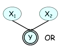
For example, consider a Bayesian network where a random variable is the OR of two other random variables, as shown in Figure 1. Initially, x1 and x2 are independent. If we observe y = 1, they become dependent because if x1 = 0 we can infer the value of x2 (and vice-versa).
On the other hand, if y =0, the variables are independent because independent of the value of the other variable, we know that the value of x1 and x2 will be 0.
We can think of this kind of context-specific independence as a special case of conditional independence. In the latter, for there to be independence, there must be context-specific independence for all combinations of values of the observed variables.
Deterministic CPDs
The example above is called a deterministic CPD. In such cases, the children’s values can be computed deterministically from its parents and hence we don’t need to include it in the combinations table.
CPD with Tree Structure
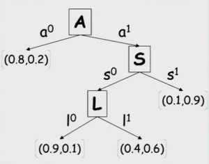
In cases where there is no conditional independence between two variables, but there is context-specific independence, we can use a tree representation instead of a table since the number of possible combinations are restricted, for example in Figure 2.
Multiplexer CPD
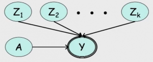
Using the tree structure, we can build a graph that represents a multiplexer, as shown in Figure 3. The variable $A$ can assume values from $1$ to $k$, while $Y$ can assume the values $Z_1, Z_2, \cdots, Z_k$. $A$ serves as the multiplexer for $Y$, by indexing the value $Z_i$. In other words, suppose $a$ is the value of $A$. Then $Y$ has value $Z_a$. The corresponding CPD for this graph is: $P(Y = Z_a \mid A = a) = 1$ and $P(Y = Z_a \mid A \neq a) = 0$ for every $1 \le a \le k$.
Noisy-OR CPD
A generalization of the deterministic CPD is the noisy CPD. This models the case where the parent variables do not include 100% the children one.
More concretely, suppose we have variable $X$ that influences $Y$, but not 100% due to some noise. If $X = 1$, then $Y = 1$ but with probability $\lambda$, or $Y = 0$ with probability $1 - \lambda$. If $X = 0$ then $Y = 0$ with 100% chance.
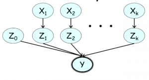
What if we have multiple $X$s each of which can affect the outcome of $Y$? To model this case, we add a “layer” of variables $Z_1, \cdots, Z_k$, where each $Z_i$ is binary, being 1 if and only if, the variable $X_k = 1$ would have set $Y = 1$.
We can also add a variable $Z_0$ to model the fact that $Y$ can be caused by something other than the variables $X$. In this model, $Y$ a deterministic OR of $Z_0, \cdots, Z_k$, as shown in Figure 4.
The CPDs of the variables $Z_k$ for $k > 0$ are $P(Z_k = 1 \mid X_k = 0) = 0$ and $P(Z_k = 1 \mid X_k = 1) = \lambda_k$, where $\lambda_k$ is the noise associated with $X_k$.
$Y$ itself is now deterministically dependent of the $Z$s via the deterministic OR. Thus, it is possible to write the CPD of $Y$ as a function of $X_1, \cdots, X_k$. Since for $Y = 0$ all $Z$s must be 0, we have:
\[P(Y = 0 \mid X_1, \cdots, X_k) = \prod_{i} P(Z_k = 0 \mid X_i)\]Since $P(Z_k = 1 \mid X_k = 0) = 1$ and $P(Z_k = 0 \mid X_k = 1) = 1 - \lambda_k$ we have
\[P(Y = 0 \mid X_1, \cdots, X_k) = (1 - \lambda_0) \prod_{i \mid X_i = 1} (1 - \lambda_i)\]CPDs for the Continuous Case
If a given variable $Y$ depends on a continuous variable $X$, it is impossible to enumerate all possible values of $X$. In this case, we can define $Y$ as a probability distribution function with $X$ as a parameter.
An example is to use the Gaussian distribution for $Y$, with the mean being the observed value of $X$, say $x$, and a fixed variance, i.e. $Y \sim \mathcal{N}(x, \sigma^2)$.
If $Y$ depends on multiple continuous variables, we can for example use some kind of function of the observed values to define the mean. If $Y$ also depends on a discrete variable, we can have a mixed CPD, where the discrete variables define the rows of the table and in each row there is a distribution with different parameters.
Markov networks
Markov networks are represented by an undirected graph.
Pairwise Markov Networks
Pairwise Markov networks are a special case of Markov networks, where the relationships between variables are always pairwise and therefore we can represent them through an undirected graph.
Instead of defining factors on vertices as in the case of Bayesian networks, we define factors on edges. In this context, these factors are called compatibility functions or affine functions.
The inputs of a factor between two variables $X_i, X_j$, which we denote by $\phi(X_i, X_j)$, are the possible combinations of the values of the variables involved.
Taking the product of the factors of the graph, we get
\[\tilde P(X_1, \cdots, X_k) = \prod_{(X_i, X_j) \in E} \phi(X_i, X_j)\]which is a non-normalized measure. Let $Z$ be the normalization constant (also known as partition function, a term inherited from statistical physics), then we can define the probability distribution function:
\[P(X_1, \cdots, X_k) = \tilde P(X_1, \cdots, X_k)/Z\]One observation is that there is no intuitive correspondence between the factors and the probability distribution $P$ for Markov networks as opposed to Bayesian networks.
This model is not very expressive. To get an idea, consider a set of $n$ random variables with $d$ possible values each. Even if we have a complete graph, with $O(n^2)$ edges and each having $O(d^2)$ entries, the distribution function will have $O(n^2d^2)$ entries, whereas it’s possible for a distribution function to have $O(d^n)$ entries.
General Gibbs distribution
The weakness of the previous model lies in the restriction of factors to only two variables. To remedy this, we can use the general Gibbs distribution, which is a generalization of pairwise Markov networks. In this case, edges can be incident to more than two vertices, as in a hypergraph.
More formally, we have a set of factors $\Phi = {\phi_1(D_1), \cdots, \phi_k(D_k)}$ where each $D_i$ is the set of random variables included in the factor $\phi_i$, and is called the domain. Taking the product of the factors of the graph, we get
\[\tilde P_{\Phi}(X_1, \cdots, X_k) = \prod_{i = 1}^{k} \phi(D_i)\]The partition function is the sum over the product for all possible combination of $X_1, \cdots, X_k$:
\[Z_{\Phi}(X_1, \cdots, X_k) = \sum_{X_1, \cdots, X_k} \tilde P_{\Phi}(X_1, \cdots, X_k)\]The general Gibbs distribution is then the probability distribution
\[P_{\Phi}(X_1, \cdots, X_k) = \frac{1}{Z_{\Phi}(X_1, \cdots, X_k)} \prod_{i = 1}^{k} \phi(D_i)\]Induced Markov network. denoted by $H_{\Phi}$, is a pairwise Markov network with a set of vertices corresponding to the union of the factor domains in $\Phi$ and there is an edge between two variables $X_i$ and $X_j$ if $X_i, X_j \in D_i$ for some $\phi_i \in \Phi$.
With this, we can present the definition of factorization for Markov networks.
Factorization. A probability distribution $P$ factors a Markov network $H$ if there is a set of factors $\Phi = {\phi_1(D_1), \cdots, \phi(D_k)}$ such that
- (1) $P = P_{\Phi}$
- (2) $H = H_\Phi$
Note that information is lost when we represent the factors by an induced Markov network and therefore we cannot recover $\Phi$ from $H_\Phi$.
However, the influence relationship between variables for a Gibbs distribution can be represented by $H_\Phi$. For this, we define the active path as a path in this graph without any observed variables. Thus, we say that one random variable influences the other if there is some active path between them in the graph $H_\Phi$.
Conditional Random Fields
Conditional Random Fields or CRFs are similar to a Gibbs distribution, except that normalization is done differently. In this case, we calculate the normalization constant by accounting only for the random variables that have the observed value. The distribution obtained after normalization is conditioned by the value of the observed variables $X$.
More formally, the normalization constant for a given set of observed random variables $X$, and a set of unobserved random variables $Y$ is equal to
\[Z_{\Phi}(X) = \sum_{Y} \tilde P_{\Phi}(X, Y)\]So we have a conditional distribution:
\[P_{\Phi}(Y \mid X) = \dfrac{\tilde P_{\Phi}(X, Y)}{Z_{\Phi}(X)}\]Logistic model. is a particular case of CRF, where we have a variable $Y$ connected to a set of variables $X = X_1, \cdots, X_k$ and where the factor of each $(Y, X_i)$ is given by
\[\phi_i(X_i, Y) = \exp(w_i 1\{X_i = 1, Y = 1\})\]where $1{X_i = 1, Y = 1}$ is an indicator function, which returns 1 if the variables have the indicated values or 0 otherwise. Thus, for $Y = 1$, $\phi_i(X_i, Y = 1) = \exp(w_i X_i)$ and for $Y = 0$, $\phi_i(X_i, Y = 0) = \exp(0) = 1$.
In this case, the product of the factors is:
\[(1) \quad \tilde P(X, Y = 1) = \prod_{i = 1}^{k} \phi_i(D_i) = \exp(\sum_i (w_i X_i))\]And
\[(2) \quad \tilde P(X, Y = 0) = 1\]The probability distribution of $Y = 1$ given $X$ is given by
\[P(Y = 1 \mid X) = \dfrac{\tilde P(Y = 1, X)}{\tilde P(Y = 1, X) + \tilde P(Y = 0, X)}\]Replacing the values of (1) and (2) we get:
\[P(Y = 1 \mid X) = \dfrac{\exp(\sum_i (w_i X_i))}{1+ \exp(\sum_i (w_i X_i))}\]Independence in Markov networks
In the same way that we have the $d$-separation in Bayesian networks, we have the separation between two variables $X$ and $Y$ in a Markov network $H$ given $Z$, denoted by $\mbox{sep}_H(X, Y \mid Z)$, which occurs when there is no active path between them given $Z$.
Lemma 1. If $P$ factors a Markov network $H$ and $\mbox{sep}_H(X, Y \mid Z)$, then $P \models (X \perp Y \mid Z)$.
In the same way as for Bayesian networks, we can define the set of conditional independences on $H$ as
\[I(H) = \{(X \perp Y \mid Z) : \mbox{sep}_H(X, Y \mid Z) \}\]If $P$ satisfies all conditional independences of $I(H)$, we say that $H $is an $I$-map (independence map) of $P$. Therefore, using Lemma 1, we have
Theorem. $P$ factors a Markov network $H$, so $H$ is an $I$-map of $P$.
Conversely, we have an almost symmetrical result:
Hammersley Clifford’s Theorem. Given a positive distribution $P$, if $H$ is an $I$-map of $P$, then $P$ factors $H$.
I-maps and perfect maps
Note: this section applies to both Bayesian and Markov networks.
We can define a set of conditional independences on $P$ (rather than a graph) as
\[I(P) = \{(X \perp Y \mid Z) : P \models (X, Y \mid Z) \}\]Note that if $P$ factors a network $G$, then $I(G) \subseteq I(P)$, but the reverse is not true.
A more sparse graph tends to contain more independence and therefore more accurately represents the independence of $P$. For this, we can remove redundant edges until obtaining a minimal $I$-map, that is, a graph for which there is no edge $(X,Y)$ such that $E(G) \setminus (X, Y)$ is an $I$-map.
Ideally, we would like to find a graph such that $I(G) = I(P)$, characterizing a perfect $I$-map, but not every distribution admits such a map. We also have the case that a distribution admits a perfect $I$-map using Bayesian networks (directed graph), but not using Markov networks (undirected graph). A simple example is the $V$ structure.
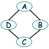
The opposite can also happen. It is not possible to capture exactly the independence of a Markov network like the one in Figure 5, in the case $(A \perp C \mid B, D)$ and $(B \perp D \mid A, C)$.
One last definition: Two graphs $G_1$ and $G_2$ are said to be $I$-equivalent if $I(G_1) = I(G_2)$.
Log-Linear Models
These models have the following form:
\[\tilde P = \exp(-\sum_j w_j f_j(D_j))\]where $w_j$ are called coefficients and $f_j()$ features, with a domain $D_j$, which is a set of random variables.
This model is quite expressive, so we can represent factors with it. If, for example, the factor $\phi$ has two random variables $X$ and $Y$ as its domain, such that $\phi(X = x_i, Y = y_j) = \sigma_{ij}$, we use an indicator function to define the characteristic function $f_{ij} = 1(X = x_i, Y = y_i)$ and coefficient $w_{ij} = \ln(\sigma_{ij})$.
But the interesting thing is that we can only model values of variables that are related (using tables, we would have multiple entries with value 0), as in the case of natural language processing. We can define a characteristic function that returns 1 if and only if a word starts with a capital letter and the label is person. The corresponding coefficient captures the correlation between these two values.
