kuniga.me > NP-Incompleteness > Open Shading Language
Open Shading Language
15 May 2011
The first step of my project is to study the Open Shading Language (OSL). In this post we will make a quick introduction to this language, according to what I have studied so far. My main sources of information are the introductory text [1], the language specification [2] and the source code itself [3].
In early 2010 Sony made the OSL code public. The language has some features that make it attractive to be used in conjunction with ray tracers. Chief among these seems to be the concept of closures. At each point on a surface, an equation may have to be solved several times to calculate what color a ray of light with a given direction will have.
The idea is that a closure stores the equation without solving for the variables. Then it can solve it later for a given input direction to get the desired color. The idea is that by doing lazy evaluation the system can be made more efficient.
Language Specification
The language specification is detailed and with examples. A very simple shader is written in OSL as follows:
shader gamma (
color Cin = 1,
float gam = 1,
output color Cout = 1
) {
Cout = pow(Cin, 1/gam);
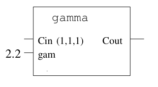
}Note that it is effectively a function, which takes some input and output parameters (which are indicated by the output keyword). We can then treat this function as a black box, as shown in Figure 1.
We can then create complex graphs of shaders, called shader groups, from individual shaders, as shown in Figure 2.
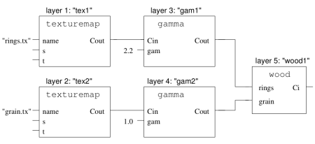
Each node of the graph above is called a shader layer. To create this graph, we declare the shaders and their connections. For the example in the figure above:
ShaderGroupBegin();
/* Nodes */
Shader(
  "texturemap", /* Shader name */
  "tex1", /* Layer (instance) name */
  "string name", "rings.tx" /* Input parameters */
);
Shader ("texturemap", "tex2", "string name", "grain.tx");
Shader("gamma", "gam1", "float gam", 2.2);
Shader("gamma", "gam2", "float gam", 1);
Shader("wood", "wood1");
/* Edges */
ConnectShaders("tex1", "Cout", "gam1", "Cin");
ConnectShaders("tex2", "Cout", "gam2", "Cin");
ConnectShaders("gam1", "Cout", "wood1", "rings");
ConnectShaders("gam2", "Cout", "wood1", "grain")
ShaderGroupEnd();
Ray tracing
After reading the language specification, the hard part began! There is little documentation on how to use OSL, being restricted to the source code itself. The first step, compiling, was already complicated. I even wrote a post describing the adaptations I had to make to be able to compile on my system.
There is a mailing list of OSL developers. The problem is that it is difficult to get help there, as hardly anyone answers anything.
Digging through the files on this list, I found an implementation of a ray tracer that uses OSL, developed by Erich Ocean and a Brecht Van Lommel, based on smallpt by Kevin Beason.
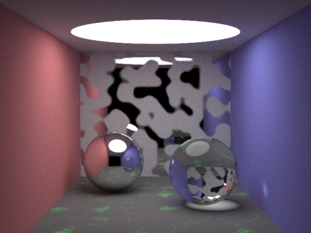
The scene we used contains spheres with different textures with a light source on top. Figure 3 is a rendered image of this scene, with 100 samples.
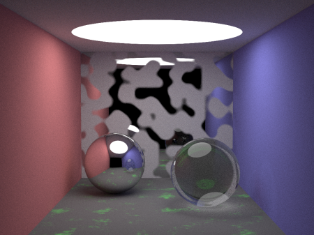
The scene actually contains 8 spheres! The apparent ones are the metal and glass balls. The walls are modeled with 5 giant spheres, so that their visible portion in the scene appears to be flat. The light on the ceiling is also a sphere, of the emissive type.
Note that the light on the glass sphere is not correct. Apparently it was a problem with the normal one, Brecht himself sent a patch with the fix, but when I applied it to my code, I got Figure 4.
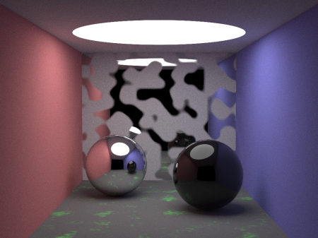
The correct image should be like Figure 5.
Unfortunately, I still haven’t figured out the reason for the error, but I’m investigating…
Studying the code
A good way to familiarize myself with the OSL language and its shader system is to play around with this ray tracer a bit. The way the algorithm generates an image from a 3D scene can be simplified as shown in Figure 6.
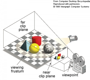
The rectangular pyramid with the top cut off is known as a frustum. The near clip plane in Figure 6 is the 2D rendered image.
Let’s describe the steps of the algorithm at a high level:
- Load shaders into memory
- Adjust camera parameters (e.g. direction the camera is point to and its position)
- For each pixel in the near clip plane, we must get its color via ray tracing
- Free the memory of everything that was allocated
- Export the image
Obviously, Step 3 is the main part of the algorithm, so let’s detail it a bit more. We divide the near clip plane into a matrix of pixels and try to determine the color for each of them.
There are infinite rays of light that can pass through a pixel in different directions, so it’s infeasible to compute them all. What is usually done is sampling: trace $s$ rays in random directions sampling that passes through that pixel.
To obtain the color, we have the following procedure called radiance:
- Identify which is the first object that the ray hits, as well as the point of intersection
- Get the shader group at the intersection point
- Evaluate the shader group’ expression
- Compute effective color for ray
Step 1 is essentially geometry. In our example, since we are dealing with spheres, it is easy to compute the points of intersection of the ray with them and then find the first object hit.
Step 2 is easy in our scene, since each sphere is associated with a unique shader group.
A shader group is associated with a closure expression, which is composed of addition and multiplication operators by a scalar or color. A closure expression is essentially a tree, and the final color is returned by a leaf (called primitive).
What the expression tree evaluator does in Step 3 is to start at the root of the tree with white color (1.0, 1.0, 1.0) and traverses the tree by choosing the children at random and then applying the corresponding operators.
A primitive can be of types: BSDF (Bidirectional Scattering Distribution Function), emissive, or background.
The color returned by Step 3 is the object’s color. The problem is that depending on the type of material, the color that is seen depends on the direction of the ray that strikes the object. Given that, Step 4 determines the actual color seen depending on the angle between the normal vector and ray.
Furthermore, we must take into account refraction and reflection, which corresponds to creating a new ray starting from the intersection point and for which we evaluate the radiance recursively. The returned color is then multiplied by the object’s color.
Next steps
According to the schedule I set up for the GSoC, I should finish studying the OSL by May 23rd. Next week I’ll try to do two things:
- Implement a shader using OSL (possibly an existing shader in BRL-CAD)
- Find the error behind the image with the black sphere. At first I’m going to download the version of the code with a date close to the one in which Brecht published the ray tracer. If it works I will check the differences between that version and the current one.
References
Notes
This is a review and translation done in 2022 of my original post in Portuguese: Open Shading Language.
