kuniga.me > NP-Incompleteness > Dijkstra And The Longest Path

Dijkstra And The Longest Path

13 Aug 2010

The shortest path problem is one of the most well-known problems in computer science. In this post, we’ll talk briefly about this problem and also the longest path problem, presenting linear programming models for both. For simplicity, we’ll assume the graph is directed and the edge weights are positive.

The Dijkstra algorithm can be used to solve the shortest path problem and was developed by Edsger Dijkstra in 1956 over coffee in a bar. The author said in a interview that it took 20 minutes to develop it!

The shortest path problem can also be modeled as a network flow. More specifically, it can be reduced to the minimum cost max flow problem where the flow out of the source is limited to 1. Working with network flow is more interesting because it’s simpler to model it as a integer linear programming as we shall see.

Let $G(V, A)$ be a directed graph with special vertices $s$ and $t$ representing the source and sink of the graph. Let $x_{ij}$ be a variable representing the amount of flow going through an arc $(i, j) \in A$.

For each node in the graph that is not the source nor sink we need the conservation of the flow:

\[\sum_{(j, i) \in E} x_{ji} = \sum_{(i, j) \in E} x_{ji} \qquad \qquad v \in V, v \neq s, t\]

The flow in each arc must be non-negative:

\[x_{ij} \ge 0 \qquad \qquad (i, j) \in A\]

Arcs can have a maximum capacity associated to it, but we can ignore it for our case. The only constraint we want to enforce is that the flow leaving the source is 1:

\[\sum_{(s, j) \in A} x_{sj} = 1\]

If arcs have an associated distance $w_{ij}$ to them, we can optimize the following objective function:

\[\min \sum_{(i, j) \in A} x_{ij} w_{ij}\]

It’s possible to show that there’s an optimal solution for this objective function where $x_{ij}$ is integral, in this case, $\curly{0, 1}$. This is a fortunate instance where the optimal value of the linear programming and the integer linear programming coincide.

It’s not hard to see that a $\curly{0,1}$ solution represents a path from $s$ to $t$ (the sequence of edges having flow equal to 1) in $G(V, A)$ and is thus a shortest path.

The Longest Path

A similar problem to the shortest path is the longest path problem. A possible application for this problem is to do a critical path analysis (CPA). It consists of building a directed graph with vertices corresponding to the activities and arcs representing the dependencies between them. That is, if there is an arc $(a, b)$, then b can only be executed after finishing $a$.

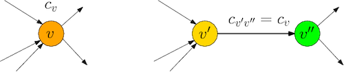
Each activity is associated with a cost, its execution time. Note that here, the cost is associated with a vertex, not an arc. This can be reduced to the one with weights on edges as follows: for each vertex $v$ and cost $w_v$, replace it with vertex $v’$ and $v’’$, then adding an edge $(v’,v’’)$ with cost $w_v$. For every arc $(v, u)$, we add arcs $(v’’, u’)$ and $(u’’, v’)$. See Figure 1 for an example.

Another characteristic of such dependency graph is that it is acyclic. Thus, it is possible to solve it in polynimial time through dynamic programming. However, for a general graph, the greatest path problem is NP-complete.

There is a property that guarantees integrality of the solution (i.e. that the PL’s solution coincides with the PLI’s) of linear programming models, which is called totally unimodularity. If the coefficient matrix of constraints of a linear program satisfies certain conditions, it is said to be totally unimodular. This implies that the problem that was modeled with this linear program can be solved in polynomial time.

Two examples of matrices that have this structure are the coefficient matrices of the PL’s of the maximum flow problem and the maximum flow with minimum cost. This means that the PL matrix of the shortest path we presented above is unimodular.

At first glance, this seems to imply that the longest path problem can be solved in polynomial time, since we just change the objective function from minimization to maximization, and since we don’t change the constraint matrix, full unimodularity is maintained.

The problem is that it is not enough just to modify the objective function for the LP to solve the maximum cost path problem. Otherwise, directed cycles of positive cost will appear, disjoint from the path of $s$ to $t$, since we want to maximize the objective function.

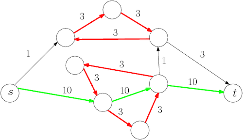
In Figure 2, the colored arcs form a feasible solution, and cycles (in red) respect flow conservation. Assuming that the capacity of the arcs is 1, the total cost of the solution below is 51. The longest path in this graph has a cost of 33, which is greater than the path found in green, which means it is not enough to throw away the cycles found to obtain an optimal solution.

In the shortest path problem they will not appear and therefore the model is valid.

Thus, it is necessary to use constraints that eliminate cycles, which unfortunately causes the constraint matrix to no longer totally unimodular. More concretelly, we define auxiliary variables $u_i$ associated with the vertices. The following restriction eliminates directed cycles:

\[(x_{ij} - 1)M + 1 \le u_j - u_i \qquad \forall (i, j) \in A\]

If flow passes through an edge it must be that $1 \le u_j - u_i$ and $u_j \gt u_i$. If there’s no flow, we have $-M + 1 \le u_j - u_i$ which is trivially satisfied.

To see that such an inequality eliminates cycles, consider a directed cycle in the graph: $(v_1, v_2), (v_2, v_3) \cdots, (v_k, v_1)$. If there’s flow in this cycle, we’ll have $u_{v_2} \gt u_{v_1}, u_{v_3} \gt u_{v_2}, \cdots u_{v_1} \gt u_{k}$, which are impossible to satisfy. Note that these can be satisfied by directed paths.